Solved Problem on Harmonic Oscillations
advertisement
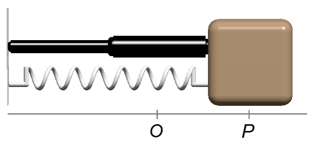
A block of mass m = 0.1 kg is connected to a spring of constant k = 0.25 N/m
and a shock absorber of damping coefficient b = 0.5 N.S/m. The block is displaced from its
equilibrium position to a point P to 0.1 m and launched with an initial speed of 0.28 m/s.
Determine:
a) Equation of displacement as a function of time;
b) What is the type of oscillation;
c) The graph of x versus t.
a) Equation of displacement as a function of time;
b) What is the type of oscillation;
c) The graph of x versus t.
Dados do problema:
- Mass of the body: m = 0.1 kg;
- Spring constant: k = 0.6 N/m;
- Damping coefficient: b = 0.5 N.s/m;
- Initial position (t = 0): x0 = 0.1 m;
- Initial velocity (t = 0): v0 = 0.28 m.
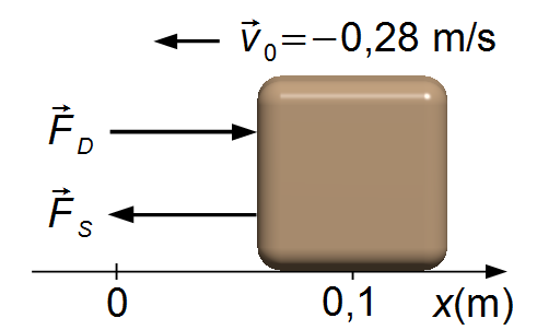
We choose a frame of reference with a positive direction to the right. The block is displaced to
position x0 = 0.1 m and when launched the elastic force will return the block to
the equilibrium position. The initial velocity points in the opposite direction of the reference
frame, v0 = −0.28 (Figure 1). Writing the Initial Conditions of the
problem
\[
\begin{array}{l}
x(0)=0.1\;\text{m}\\[10pt]
v_{0}=\dfrac{dx(0)}{dt}=-0.28\;\text{m/s}
\end{array}
\]
Solution
a) Applying Newton's Second Law
\[
\begin{gather}
\bbox[#99CCFF,10px]
{F=m\frac{d^{2}x}{dt^{2}}} \tag{I}
\end{gather}
\]
the spring force is given by
\[
\begin{gather}
\bbox[#99CCFF,10px]
{F_{S}=-kx} \tag{II-a}
\end{gather}
\]
the damping force is given by
\[
\begin{gather}
\bbox[#99CCFF,10px]
{F_{D}=-bv=-b\frac{dx}{dt}} \tag{II-b}
\end{gather}
\]
the negative sign in spring force indicates that it acts in the opposite direction of the block
displacement (acts to restore the equilibrium), in the damping force indicates that it acts in the
opposite direction of the velocity (acts to brake the movement). Substituting the expressions (II-a)
and (II-B) into expression (I)
\[
\begin{gather}
-F_{E}-F_{R}=m\frac{d^{2}x}{dt^{2}}\\[5pt]
-kx-b\frac{dx}{dt}=m\frac{d^{2}x}{dt^{2}}\\[5pt]
m\frac{d^{2}x}{dt^{2}}+b\frac{dx}{dt}+kx=0
\end{gather}
\]
this is a Second-Order Linear Homogeneous Differential Equation. Dividing the equation by the
mass m
\[
\begin{gather}
\frac{d^{2}x}{dt^{2}}+\frac{b}{m}\frac{dx}{dt}+\frac{k}{m}x=0
\end{gather}
\]
substituting the values given in the problem
\[
\begin{gather}
\frac{d^{2}x}{dt^{2}}+\frac{0.5}{0.1}\frac{dx}{dt}+\frac{0.6}{0.1}x=0\\[5pt]
\frac{d^{2}x}{dt^{2}}+5\frac{dx}{dt}+6x=0 \tag{III}
\end{gather}
\]
Solution of
\( \displaystyle \frac{d^{2}x}{dt^{2}}+5\frac{dx}{dt}+6x=0 \)
The solution to this type of equation is found by substituting
Differentiating the expression (IV) with respect to time
The solution to this type of equation is found by substituting
\[
\begin{array}{l}
x=\operatorname{e}^{\lambda t}\\[5pt]
\dfrac{dx}{dt}=\lambda \operatorname{e}^{\lambda t}\\[5pt]
\dfrac{d^{2}x}{dt^{2}}=\lambda^{2}\operatorname{e}^{\lambda t}
\end{array}
\]
substituting these values in the differential equation
\[
\begin{gather}
\lambda^{2}\operatorname{e}^{\;\lambda t}+5\lambda \operatorname{e}^{\lambda t}+6\operatorname{e}^{\lambda t}=0\\[5pt]
\operatorname{e}^{\lambda t}\left(\lambda^{2}+5\lambda +6\right)=0\\[5pt]
\lambda^{2}+5\lambda +6=\frac{0}{\operatorname{e}^{\lambda t}}\\[5pt]
\lambda^{2}+5\lambda +6=0
\end{gather}
\]
this is the Characteristic Equation that has the solution
\[
\begin{array}{l}
\Delta =b^{2}-4ac=5^{2}-4\times 1\times 6=25-24=1\\
\lambda=\dfrac{-b\pm\sqrt{\Delta\;}}{2a}=\dfrac{-5\pm\sqrt{1\;}}{2\times 1}=\dfrac{-5\pm1}{2}\\[10pt]
\lambda_{1}=-2 \qquad \text{e} \qquad \lambda_{2}=-3
\end{array}
\]
The solution of the differential equation will be
\[
\begin{gather}
x=C_{1}\operatorname{e}^{\lambda_{1}t}+C_{2}\operatorname{e}^{\lambda_{2}t}\\[5pt]
x=C_{1}\operatorname{e}^{-2t}+C_{2}\operatorname{e}^{-3t} \tag{IV}
\end{gather}
\]
where C1 and C2 are constant of integration determined by the
Initial Cconditions.Differentiating the expression (IV) with respect to time
\[
\begin{gather}
\frac{dx}{dt}=-2C_{1}\operatorname{e}^{-2t}-3C_{2}\operatorname{e}^{-3t} \tag{V}
\end{gather}
\]
Substituting the Initial Conditions into expressions (IV) and (V)
\[
\begin{gather}
x(0)=0.1=C_{1}\operatorname{e}^{-2.0}+C_{2}\operatorname{e}^{-3.0}\\[5pt]
0.1=C_{1}\operatorname{e}^{0}+C_{2}\operatorname{e}^{0}\\[5pt]
0.1=C_{1}+C_{2} \tag{VI}
\end{gather}
\]
\[
\begin{gather}
\frac{dx(0)}{dt}=-0.28=-2C_{1}\operatorname{e}^{-2.0}-3C_{2}\operatorname{e}^{-3.0}\\[5pt]
-0.28=-2C_{1}\operatorname{e}^{0}-3C_{2}\operatorname{e}^{0}\\[5pt]
-0.28=-2C_{1}-3C_{2} \tag{VII}
\end{gather}
\]
The expressions (VI) and (VII) can be written as a system of two equations with two unknowns
(C1 and C2)
\[
\left\{
\begin{array}{l}
C_{1}+C_{2}=0.1\\[5pt]
-2C_{1}-3C_{2}=-0.28
\end{array}
\right.
\]
solving the first equation for C1 and substituting it into the second equation
\[
\begin{gather}
C_{1}=0.1-C_{2} \tag{VIII}
\end{gather}
\]
\[
\begin{gather}
-2\left(0.1-C_{2}\right)-3C_{2}=-0.28\\[5pt]
-0.2+2C_{2}-3C_{2}=-0.28\\[5pt]
-C_{2}=-0.2+0.2\\[5pt]
-C_{2}=-0.08\\[5pt]
C_{2}=0.08
\end{gather}
\]
substituting the value of C2 into the expression (VIII)
\[
\begin{gather}
C_{1}=0.1-0.08\\[5pt]
C_{1}=0.02
\end{gather}
\]
substituting these constants into the expression (IV)
\[
x(t)=0.02\operatorname{e}^{-2t}+0.08\operatorname{e}^{-3t}
\]
\[
\begin{gather}
\bbox[#FFCCCC,10px]
{x(t)=0.02\operatorname{e}^{-2t}+0.08\operatorname{e}^{-3t}}
\end{gather}
\]
b) As Δ > 0 the oscillator is overdamped.
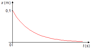
c) Plotting the graph of
\[
\begin{gather}
x(t)=0.02\operatorname{e}^{-2t}+0.08\operatorname{e}^{-3t} \tag{IX}
\end{gather}
\]
Setting x(t) = 0, we find the roots of the equation
Differentiation of the expression (IX)
The second derivative of the function
Setting t = 0 in the expression (IX)
\[
\begin{gather}
x(t)=0.02\operatorname{e}^{-2t}+0.08\operatorname{e}^{-3t}=0\\[5pt]
0.02\operatorname{e}^{-2t}=-0.08\operatorname{e}^{-3t}\\[5pt]
\frac{\operatorname{e}^{-2t}}{\operatorname{e}^{-3t}}=-{\frac{0.08}{0.02}}\\[5pt]
\operatorname{e}^{-2t}\operatorname{e}^{3t}=-4\\[5pt]
\operatorname{e}^{-2t+3t}=-4\\[5pt]
\operatorname{e}^{t}=-4
\end{gather}
\]
no t satisfies the equality, the function x(t) does not cross the t-axis. For
any real value of t, the function will always be positive, x(t) > 0,
the graph will always be obove the t-axis.Differentiation of the expression (IX)
\[
\begin{gather}
\frac{dx}{dt}=(-2)\times 0.02\operatorname{e}^{-2t}+(-3)\times 0.08\operatorname{e}^{-3t}\\[5pt]
\frac{dx}{dt}=-0.04\operatorname{e}^{-2t}-0.24\operatorname{e}^{-3t} \tag{X}
\end{gather}
\]
for any real value of t, the derivative will always be negative
\( \left(\dfrac{dx(t)}{dt}<0\right) \)
and the function decreases. Setting
\( \dfrac{dx(t)}{dt}=0 \),
we find the maximum and minimum points of the function.
\[
\begin{gather}
\frac{dx}{dt}=-0.04\operatorname{e}^{-2t}-0.24\operatorname{e}^{-3t}=0\\[5pt]
0.04\operatorname{e}^{-2t}=-0.24\operatorname{e}^{-3t}\\[5pt]
\frac{\operatorname{e}^{-2t}}{\operatorname{e}^{-3t}}=-{\frac{0.24}{0.04}}\\[5pt]
\operatorname{e}^{-2t}\operatorname{e}^{3t}=-6\\[5pt]
\operatorname{e}^{-2t+3t}=-6\\[5pt]
\operatorname{e}^{t}=-6
\end{gather}
\]
no t that satisfies this equality, there are no maximum or minimum points of the function.The second derivative of the function
\[
\begin{gather}
\frac{d^{2}x}{dt^{2}}=-(-2)\times 0.04\operatorname{e}^{-2t}-(-3)\times 0.24\operatorname{e}^{-3t}\\[5pt]
\frac{d^{2}x}{dt^{2}}=0.08\operatorname{e}^{-2t}+0.72\operatorname{e}^{-3t} \tag{XI}
\end{gather}
\]
for any real value t, the second derivative will always be positive
\( \left(\dfrac{d^{2}x(t)}{dt^{2}}>0\right) \)
and the function is concave upwards. Setting
\(\dfrac{d^{2}x(t)}{dt^{2}}=0 \)
we find inflection points in the function.
\[
\begin{gather}
\frac{d^{2}x}{dt^{2}}=0.08\operatorname{e}^{-2t}+0.72\operatorname{e}^{-3t}=0\\[5pt]
0.08\operatorname{e}^{-2t}=-0.72\operatorname{e}^{-3t}\\[5pt]
\frac{\operatorname{e}^{-2t}}{\operatorname{e}^{-3t}}=-{\frac{0.72}{0.08}}\\[5pt]
\operatorname{e}^{-2t}.\operatorname{e}^{-3t}=-9\\[5pt]
\operatorname{e}^{-2t+3t}=-9\\[5pt]
\operatorname{e}^{t}=-9
\end{gather}
\]
as there is no t that satisfies this equality, there are no inflection points in the function.Setting t = 0 in the expression (IX)
\[
\begin{gather}x(0)=0.02\operatorname{e}^{-2.0}+0.08\operatorname{e}^{-3.0}\\[5pt]
x(0)=0.02\operatorname{e}^{0}+0.08\operatorname{e}^{0}\\[5pt]
x(0)=0.02+0.08\\[5pt]
x(0)=0.1
\end{gather}
\]
As the variable t represents time, we do not calculate negative values, t < 0, for
t tending to infinity
\[
\begin{split}
\lim_{t\rightarrow \infty }x(t) &=\lim _{t\rightarrow\infty}\left[0.02\operatorname{e}^{-2t}+0.08\operatorname{e}^{-3t}\right]=\\[5pt]
&=\lim_{t\rightarrow \infty}\left[\frac{0.02}{\operatorname{e}^{2t}}+\frac{0.08}{\operatorname{e}^{3t}}\right]=\\[5pt]
&=\frac{0.02}{\operatorname{e}^{2\times\infty}}+\frac{0.08}{\operatorname{e}^{3\times\infty }}=0+0=0
\end{split}
\]
From the above analysis, we plot the graph of x versus t (Graph 2).
advertisement

Fisicaexe - Physics Solved Problems by Elcio Brandani Mondadori is licensed under a Creative Commons Attribution-NonCommercial-ShareAlike 4.0 International License .