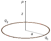
A ring of radius a carries a uniformly distributed electric charge q₁ on one half and q₂ on the other half. Calculate the electric field vector at point P on the symmetry axis perpendicular to the plane of the ring at a distance z from its center.

Problem data:

• Radius of the ring:    a;
• Charge in one half of the ring:    q₁;
• Charge in the other half of the ring:    q₂;
• Distance to the point where we want the electric field:    z.

Solution:

• For the half of the ring with charge q₁ between 0 and π.

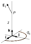
The position vector r₁ goes from an element of charge dq₁ to point P, where we want to calculate the electric field, the vector r_q locates the charge element relative to the origin of the reference frame, and the vector r_p locates point P (Figure 1-A).

Figure 1

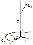
From the geometry of the problem, we choose cylindrical coordinates (Figure 1-B), the r_q vector, which is on the xy plane, is written as   \( {\mathbf{r}}_{q}=x\;\mathbf{i}+y\;\mathbf{j} \),   and the r_p vector only has a component in the k direction,   \( {\mathbf{r}}_{p}=z\;\mathbf{k} \),   the position vector will be

From expression (I), the magnitude of the position vector r₁ will be

where x, y, and z, in cylindrical coordinates, are given by

The electric field vector of this half of the ring is given by

Using the expression of the linear density of charge λ₁, we have the charge element dq₁.

\[ \begin{gather} \bbox[#99CCFF,10px] {\lambda=\frac{dq}{ds}} \end{gather} \]

\[ \begin{gather} \lambda_1=\frac{dq_1}{ds_1} \\[5pt] dq_1=\lambda_1\;ds_1 \tag{V} \end{gather} \]

Figure 2

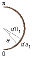
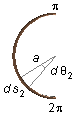
where ds₁ is an arc element with angle dθ₁ (Figure 2).

substituting the expression (VI) into expression (V).

Substituting expressions (I), (II), and (VII) into expression (IV).

substituting expressions (III) into expression (VIII).

As the charge density λ₁ and the radius a are constants, they are moved outside the integral, and the integral of the sum is equal to the sum of the integrals.

The limits of integration, for this half of the ring, will be 0 and π (half-turn - Figure 2).

Integration of    \( \displaystyle \int_{0}^{\pi }\cos\theta_{1}\;d\theta_{1} \)

1st method

\[ \begin{align} \int_0^{\pi}\cos\theta_1\;d\theta_1 &=\left.\sin \theta_1\;\right|_{\;0}^{\;\pi}=\sin \pi -\sin 0=\\ &=0-0=0 \end{align} \]

2nd method

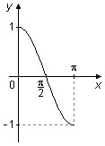
The graph of cosine between 0 and π has a "positive" area above the x-axis between 0 and \( \frac{\pi}{2} \), and a "negative" area below the x-axis, between \( \frac{\pi}{2} \) and π, these two areas cancel in the integration, and the integral is equal to zero (Figure 3).

Figure 3

\[ \begin{gather} {\mathbf E}_1=\frac{1}{4\pi \epsilon_0}\;\frac{\lambda_1a}{\left(a^2+z^2\right)^{3/2}}\left(-a\times 0\;\mathbf i-2a\;\mathbf j+\pi z\;\mathbf k\right) \\[5pt] {\mathbf E}_1=\frac{1}{4\pi\epsilon_0}\;\frac{\lambda_1a}{\left(a^2+z^2\right)^{3/2}}\left(-2a\;\mathbf j+\pi z\;\mathbf k\right) \tag{IX} \end{gather} \]

Figure 4

• For the half of the ring with charge q₂ between π and 2π.

From the expression of linear density of charges (V), we have the element of charge dq₂.

\[ \begin{gather} dq_2=\lambda_2\;ds_2 \tag{XI} \end{gather} \]

substituting the expressions (I), (II), and (XI) into expression (X), we have a similar result to expression (VIII).

\[ \begin{gather} {\mathbf E}_2=\frac{1}{4\pi \epsilon_0}\int{\frac{\lambda_2a\;d\theta_2}{\left(x^2+y^2+z^2\right)^{3/2}}}\left(-x\;\mathbf i-y\;\mathbf j+z\;\mathbf k\right) \tag{XII} \end{gather} \]

Figure 5

substituting expressions (III) into expression (XII) and following the same algebraic manipulation.

The limits of integration, for this half of the ring, will be π and 2π (half-turn - Figure 5).

Integration of    \( \displaystyle \int_{\pi}^{{2\pi}}\cos\theta_2\;d\theta_2 \)

1st method

\[ \begin{align} \int_{\pi}^{{2\pi}}\cos\theta_2\;d\theta_2 &=\left.\sin \theta_2\;\right|_{\;\pi }^{\;2\pi}=\sin 2\pi -\sin \pi =\\ &=0-0=0 \end{align} \]

2nd method

The graph of cosine between π and 2π has a "negative" area below the x-axis between π and \( \frac{3\pi}{2} \), and a "positive" area above the x-axis between \( \frac{3\pi}{2} \) and 2π, these two areas cancel in the integration, and the integral is equal to zero (Figure 6).

Figure 6

\[ \begin{gather} {\mathbf E}_2=\frac{1}{4\pi\epsilon_0}\;\frac{\lambda_2a}{\left(a^2+z^2\right)^{3/2}}\left[-a\times 0\;\mathbf i-(-2)a\;\mathbf j+\pi z\;\mathbf k\right] \\[5pt] {\mathbf E}_2=\frac{1}{4\pi\epsilon_0}\;\frac{\lambda_2a}{\left(a^2+z^2\right)^{3/2}}\left(2a\;\mathbf j+\pi z\;\mathbf k\right) \tag{XIII} \end{gather} \]

Figure 7

The total electric field vector is given by the sum of the expressions (IX) and (XIII).

The charges of each half of the ring are q₁ and q₂, and their lengths are πa, the linear density of charges of each half will be

substituting these expressions into expression (XIV).

Note: If the charge q₁ is greater than the charge q₂, the term in the j direction will be negative \( q_2-q_1<0 \), and the electric field vector is in the directions −j and k (Figure 8-A). If the charge q₁ is less than the charge q₂, the term in the j direction will be positive, \( q_2-q_1>0 \), and the electric field vector is in the directions +j and k (Figure 8-B). If q₁ and q₂ charges are equal to \( \left(q_1=q_2=\frac{Q}{2}\right) \), each half of the ring has half of the charge \( \frac{Q}{2} \), then the electric field vector expression

Figure 8

\[ \begin{gather} \mathbf E=\frac{1}{4\pi\epsilon_0}\frac{a}{\left(a^2+z^2\right)^{3/2}}\left[\frac{2}{\pi}\underbrace{\left(\frac{Q}{2}-\frac{Q}{2}\right)}_0\;\mathbf j+\frac{z}{a}\underbrace{\left(\frac{Q}{2}+\frac{Q}{2}\right)}_{Q}\;\mathbf k\right] \\[5pt] \mathbf E=\frac{1}{4\pi\epsilon_0}\frac{a}{\left(a^2+z^2\right)^{3/2}}\left[\frac{2}{\pi}\times 0\;\mathbf j+\frac{z}{a}Q\;\mathbf k\right] \\[5pt] \mathbf E=\frac{1}{4\pi\epsilon_0}\frac{\cancel{a}}{\left(a^2+z^2\right)^{3/2}}\frac{z}{\cancel{a}}Q\;\mathbf k\\[5pt] \mathbf E=\frac{1}{4\pi\epsilon_0}\frac{Qz}{\left(a^2+z^2\right)^{3/2}}\;\mathbf k \end{gather} \]

and so the result is obtained for the electric field vector of a ring of uniform charge. (Figure 8-C).