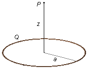
A ring of radius a carries a uniformly distributed electric charge Q. Calculate the
electric field vector at point P on the symmetry axis perpendicular to the plane of the ring
at a distance z from its center.
Problem data:
- Radius of the ring: a;
- Charge of the ring: Q;
- Distance to the point where we want the electric field: z.
Problem diagram:
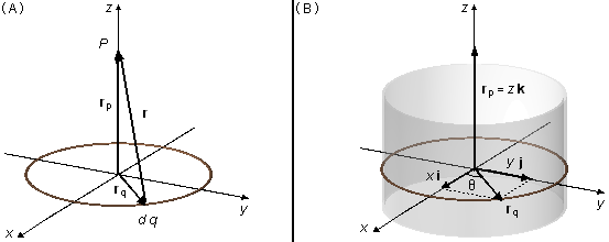
The position vector r goes from an element of charge dq to point P, where we want to
calculate the electric field, the vector rq locates the charge element relative to
the origin of the reference frame, and the vector rp locates point P
(Figure 1-A).
\[
\begin{gather}
\mathbf r=\mathbf r_p-\mathbf r_q
\end{gather}
\]
From the geometry of the problem, we choose cylindrical coordinates (Figure 1-B). The vector
rq is on the xy plane, it is written as
\( \mathbf r_q=x\;\mathbf i+y\;\mathbf j \).
The vector rp only has a component in the k direction,
\( \mathbf r_p=z\;\mathbf k \),
the position vector will be
\[
\begin{gather}
\mathbf r=z\;\mathbf k-\left(x\;\mathbf i+y\;\mathbf j\right)\\[5pt]
\mathbf r=-x\;\mathbf i-y\;\mathbf j+z\;\mathbf k \tag{I}
\end{gather}
\]
From equation (I), the magnitude of the position vector r will be
\[
\begin{gather}
r^2=(-x)^2+(-y)^2+z^2\\[5pt]
r=\left(x^2+y^2+z^2\right)^{\frac{1}{2}} \tag{II}
\end{gather}
\]
where x, y, and z, in cylindrical coordinates, are given by
\[
\begin{gather}
\left\{
\begin{array}{l}
x=a\cos\theta\\
y=a\sin\theta\\
z=z
\end{array}
\right. \tag{III}
\end{gather}
\]
Solution:
The electric field vector is given by
\[
\begin{gather}
\bbox[#99CCFF,10px]
{\mathbf E=\frac{1}{4\pi\epsilon_0}\int{\frac{dq}{r^2}\;\frac{\mathbf r}{r}}}
\end{gather}
\]
\[
\begin{gather}
\mathbf E=\frac{1}{4\pi\epsilon_0}\int{\frac{dq}{r^3}\;\mathbf r} \tag{IV}
\end{gather}
\]
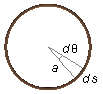
Using the equation of the linear density of charge, λ, we have the charge element dq.
\[
\begin{gather}
\bbox[#99CCFF,10px]
{\lambda =\frac{dq}{ds}}
\end{gather}
\]
\[
\begin{gather}
dq=\lambda\;ds \tag{V}
\end{gather}
\]
where
ds is an arc element with angle
dθ (Figure 2).
\[
\begin{gather}
ds=a\;d\theta \tag{VI}
\end{gather}
\]
substituting the equation (VI) into equation (V).
\[
\begin{gather}
dq=\lambda a\;d\theta \tag{VII}
\end{gather}
\]
Substituting equations (I), (II), and (VII) into equation (IV).
\[
\begin{gather}
\mathbf E=\frac{1}{4\pi\epsilon_0}\int{\frac{\lambda a\;d\theta}{\left[\left(x^2+y^2+z^2\right)^{1/2}\right]^3}}\left(-x\;\mathbf i-y\;\mathbf j+z\;\mathbf k\right)\\[5pt]
\mathbf E=\frac{1}{4\pi\epsilon_0}\int{\frac{\lambda a\;d\theta}{\left(x^2+y^2+z^2\right)^{3/2}}}\left(-x\;\mathbf i-y\;\mathbf j+z\;\mathbf k\right) \tag{VIII}
\end{gather}
\]
substituting equations (III) into equation (VIII).
\[
\begin{gather}
\mathbf E=\frac{1}{4\pi\epsilon_0}\int{\frac{\lambda a\;d\theta}{\left[\left(a\cos\theta\right)^2+\left(a\sin\theta\right)^2+z^2\right]^{3/2}}}\left(-a\cos\theta\;\mathbf i-a\sin\theta\;\mathbf j+z\mathbf k\right)\\[5pt]
\mathbf E=\frac{1}{4\pi\epsilon_0}\int{\frac{\lambda a\;d\theta}{\left[a^2\cos^2\theta +a^2\sin^2\theta+z^2\right]^{3/2}}}\left(-a\cos\theta\;\mathbf i-a\sin\theta\;\mathbf j+z\;\mathbf k\right)\\[5pt]
\mathbf E=\frac{1}{4\pi\epsilon_0}\int{\frac{\lambda a\;d\theta}{\left[a^2\underbrace{\left(\cos^2\theta +\sin^2\theta\right)}_{1}+z^2\right]^{3/2}}}\left(-a\cos\theta\;\mathbf i-a\sin\theta\;\mathbf j+z\;\mathbf k\right)\\[5pt]
\mathbf E=\frac{1}{4\pi\epsilon_0}\int{\frac{\lambda a\;d\theta}{\left(a^2+z^2\right)^{3/2}}}\left(-a\cos\theta\;\mathbf i-a\sin\theta\;\mathbf j+z\;\mathbf k\;\right)
\end{gather}
\]
As the charge density λ and the radius a are constants, they are moved outside of the
integral, and the integral of the sum is equal to the sum of the integrals.
\[
\begin{gather}
\mathbf E=\frac{1}{4\pi\epsilon_0}\frac{\lambda a}{\left(a^2+z^2\right)^{3/2}}\left(-a\int\cos\theta\;d\theta\;\mathbf i-a\int\sin\theta\;d\theta\;\mathbf j+z\int\;d\theta\;\mathbf k\;\right)
\end{gather}
\]
The limits of integration will be 0 and 2π (a complete lap in the ring).
\[
\begin{gather}
\mathbf E=\frac{1}{4\pi\epsilon_0}\frac{\lambda a}{\left(a^2+z^2\right)^{3/2}}\left(-a\underbrace{\int_0^{2\pi}\cos\theta\;d\theta}_0\;\mathbf i-a\underbrace{\int_0^{2\pi}\sin\theta\;d\theta}_0\;\mathbf j+z\int_0^{2\pi}\;d\theta\;\mathbf k\right)
\end{gather}
\]
Integration of
\( \displaystyle \int_0^{2\pi}\cos\theta\;d\theta \)
1st method
\[
\begin{align}
\int_0^{2\pi}\cos\theta\;d\theta &=\left.\sin\theta\;\right|_{\;0}^{\;2\pi}=\sin2\pi-\sin0=\\
&=0-0=0
\end{align}
\]
2nd method
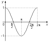
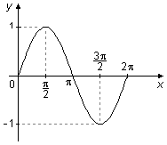
The graph of cosine between 0 and 2π has a "positive" area above the x-axis between 0 and
\( \frac{\pi}{2} \),
and between
\( \frac{3\pi}{2} \)
and 2π. And a "negative" area below the x-axis between
\( \frac{\pi}{2} \)
and
\( \frac{3\pi}{2} \),
these two areas cancel in the integration, and the integral is equal to zero (Figure 3).
Integration of
\( \displaystyle \int_0^{2\pi}\sin\theta\;d\theta \)
1st method
\[
\begin{align}
\int_0^{2\pi}\sin\theta\;d\theta &=\left.-\cos\theta\;\right|_{\;0}^{\;2\pi}=-(\cos 2\pi-\cos 0)=\\
&=-(1-1)=0
\end{align}
\]
2nd method
The graph of sine between 0 and 2π has a "positive" area above the x-axis between 0 and
π. And a "negative" area below the x-axis between π and 2π, these two areas cancel in
the integration, and the integral is equal to zero (Figure 4).
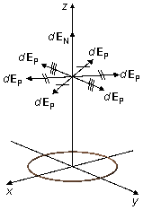
Note: The two integrals, in directions i and j, which are zero, represent
the mathematical calculation for the assertion that is usually made that the components of the
electric field parallel to the xy plane (dEP) cancel. Only the
normal components of the plane (dEN) contribute to the total electric
field (Figure 5).
Integration of
\( \displaystyle \int_0^{2\pi}d\theta \)
\[
\begin{gather}
\int_0^{2\pi}d\theta =\left.\theta\;\right|_{\;0}^{\;2\pi}=2\pi-0=2\pi
\end{gather}
\]
\[
\begin{gather}
\mathbf E=\frac{1}{4\pi\epsilon_0}\frac{\lambda a}{\left(a^2+z^2\right)^{3/2}}2\pi z\;\mathbf k\\[5pt]
\mathbf E=\frac{1}{4\pi\epsilon_0}\frac{2\pi\lambda a z}{\left(a^2+z^2\right)^{3/2}}\;\mathbf k \tag{IX}
\end{gather}
\]
The total charge of the ring is Q, and its length is 2πa, and the linear charge density
can be written as
\[
\begin{gather}
\lambda =\frac{Q}{2\pi a}\\[5pt]
Q=2\pi a\lambda \tag{X}
\end{gather}
\]
substituting equation (X) into equation (IX).
\[
\begin{gather}
\bbox[#FFCCCC,10px]
{\mathbf E=\frac{1}{4\pi\epsilon_0}\frac{Qz}{\left(a^2+z^2\right)^{3/2}}\;\mathbf k}
\end{gather}
\]