Solved Problem on Collisions
advertisement
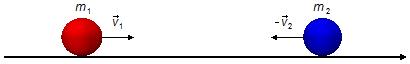
Two elastic balls, with masses m1 and m2 and speeds v1 and v2 respectively, collide head-on, their speeds are in the direction of the line joining their centers. Determine the speeds of the balls after the collision in the following cases:
a) The speed of the second ball before the impact is equal to zero;
b) The masses of the balls are equal.
Problem data:
- Mass of ball 1: m1;
- Mass of ball 2: m2;
- Initial speed of ball 1: v1;
- Initial speed of ball 2: v2.
We choose a reference frame pointing to the right, with the speed of ball 1 in the same direction as the reference frama, v1 > 0, and the speed of ball2 in the opposite direction, v2 < 0 (Figure 1).
Solution
As the collision is elastic, the momentum and kinetic energy of the system are conserved. We write the equations for balls 1 and 2 in the initial and final situations.
The momentum is given by
\[
\begin{gather}
\bbox[#99CCFF,10px]
{\vec Q=m\vec v}
\end{gather}
\]
The kinetic energy is given by
\[
\begin{gather}
\bbox[#99CCFF,10px]
{K=\frac{mv^{2}}{2}}
\end{gather}
\]
- Before the collision
\[
\begin{gather}
Q_{1i}=m_{1}v_{1} \tag{I}
\end{gather}
\]
\[
\begin{gather}
Q_{2i}=m_{2}v_{2} \tag{II}
\end{gather}
\]
\[
\begin{gather}
K_{1i}=\frac{m_{1}v_{1}^{2}}{2} \tag{III}
\end{gather}
\]
\[
\begin{gather}
K_{2i}=\frac{m_{2}v_{2}^{2}}{2} \tag{IV}
\end{gather}
\]
- After the collision
\[
\begin{gather}
Q_{1f}=m_{1}v_{1f} \tag{V}
\end{gather}
\]
\[
\begin{gather}
Q_{2f}=m_{2}v_{2f} \tag{VI}
\end{gather}
\]
\[
\begin{gather}
K_{1f}=\frac{m_{1}v_{1f}^{2}}{2} \tag{VII}
\end{gather}
\]
\[
\begin{gather}
K_{2f}=\frac{m_{2}v_{2f}^{2}}{2} \tag{VIII}
\end{gather}
\]
Applying the Law of Conservation of linear Momentum, applying equations (I), (II), (V) and (VI)
\[
\begin{gather}
Q_{i}=Q_{f}\\[5pt]
m_{1}v_{1}-m_{2}v_{2}=m_{1}v_{1f}+m_{2}v_{2f} \tag{IX}
\end{gather}
\]
Applying the Law of Conservation of Energy, applying equations (III), (IV), (VII) and (VIII)
\[
\begin{gather}
K_{i}=K_{f}\\[5pt]
\frac{m_{1}v_{1}^{2}}{\cancel{2}}+\frac{m_{2}v_{2}^{2}}{\cancel{2}}=\frac{m_{1}v_{1f}^{2}}{\cancel{2}}+\frac{m_{2}v_{2f}^{2}}{\cancel{2}}\\[5pt]
m_{1}v_{1}^{2}+m_{2}v_{2}^{2}=m_{1}v_{1f}^{2}+m_{2}v_{2f}^{2} \tag{X}
\end{gather}
\]
Equations (IX) and (X) can be written as a system of two equations with two unknowns
(v1f and v2f)
\[
\begin{gather}
\left\{
\begin{matrix}
\;m_{1}v_{1}-m_{2}v_{2}=m_{1}v_{1f}+m_{2}v_{2f}\\
\;m_{1}v_{1}^{2}+m_{2}v_{2}^{2}=m_{1}v_{1f}^{2}+m_{2}v_{2f}^{2}
\end{matrix} \tag{XI}
\right.
\end{gather}
\]
a) Letting v2 = 0 in system (XI)
\[
\begin{gather}
\left\{
\begin{matrix}
\;m_{1}v_{1}-m_{2}.0=m_{1}v_{1f}+m_{2}v_{2f}\\
\;m_{1}v_{1}^{2}+m_{2}.0^{2}=m_{1}v_{1f}^{2}+m_{2}v_{2f}^{2}
\end{matrix}
\right.
\\[5pt]
\left\{
\begin{matrix}
\;m_{1}v_{1}=m_{1}v_{1f}+m_{2}v_{2f}\\
\;m_{1}v_{1}^{2}=m_{1}v_{1f}^{2}+m_{2}v_{2f}^{2}
\end{matrix}
\right.
\end{gather}
\]
solving the first equation for v2f
\[
\begin{gather}
m_{2}v_{2f}=m_{1}v_{1}-m_{1}v_{1f}\\[5pt]
v_{2f}=\frac{1}{m_{2}}(m_{1}v_{1}-m_{1}v_{1f}) \tag{XII}
\end{gather}
\]
and substituting in the second equation
\[
\begin{gather}
m_{1}v_{1}^{2}=m_{1}v_{1f}^{2}+m_{2}\left[\frac{1}{m_{2}}(m_{1}v_{1}-m_{1}v_{1f})\right]^{2}\\[5pt]
m_{1}v_{1}^{2}=m_{1}v_{1f}^{2}+\cancel{m_{2}}\frac{1}{m_{2}^{\cancel{2}}}(m_{1}v_{1}-m_{1}v_{1f})^{2}
\end{gather}
\]
the term in parentheses on the right-hand side of the equality is a special binomial of the type
\( (a-b)^{2}=a^{2}-2ab+b^{2} \)
\[
\begin{gather}
m_{1}v_{1}^{2}=m_{1}v_{1f}^{2}+\frac{1}{m_{2}}\left(m_{1}^{2}v_{1}^{2}-2m_{1}^{2}v_{1}v_{1f}+m_{1}^{2}v_{1f}^{2}\right) \tag{XIII}
\end{gather}
\]
multiplying equation (XIII) by m2
\[
\begin{gather}
\qquad \qquad \qquad m_{1}v_{1}^{2}=m_{1}v_{1f}^{2}+\frac{1}{m_{2}}\left(m_{1}^{2}v_{1}^{2}-2m_{1}^{2}v_{1}v_{1f}+m_{1}^{2}v_{1f}^{2}\right)\qquad (\;\times m_{2}\;)\\[5pt]
\; m_{1}m_{2}v_{1}^{2}=m_{1}m_{2}v_{1f}^{2}+m_{1}^{2}v_{1}^{2}-2m_{1}^{2}v_{1}v_{1f}+m_{1}^{2}v_{1f}^{2}\\[5pt]
\; \cancel{m_{1}}m_{2}v_{1}^{2}=\cancel{m_{1}}\left( m_{2}v_{1f}^{2}+m_{1}v_{1}^{2}-2m_{1}v_{1}v_{1f}+m_{1}v_{1f}^{2}\right)\\[5pt]
m_{2}v_{1}^{2}=m_{2}v_{1f}^{2}+m_{1}v_{1}^{2}-2m_{1}v_{1}v_{1f}+m_{1}v_{1f}^{2}\\[5pt]
\left(m_{2}+m_{1}\right)v_{1f}^{2}-2m_{1}v_{1}v_{1f}+m_{1}v_{1}^{2}-m_{2}v_{1}^{2}=0
\end{gather}
\]
This is a Quadratic Equation of type
\( ax^{2}+bx+c=0 \)
where the unknown is the value v1f.
Solution ofde
\( \underbrace{\left(m_{2}+m_{1}\right)}_{a}\underbrace{v_{1f}^{2}}_{x^{2}}-\underbrace{2m_{1}v_{1}}_{b}\underbrace{v_{1f}}_{x}+\underbrace{m_{1}v_{1}^{2}-m_{2}v_{1}^{2}}_{c}=0 \)
\[ \underbrace{\left(m_{2}+m_{1}\right)}_{a}\underbrace{v_{1f}^{2}}_{x^{2}}-\underbrace{2m_{1}v_{1}}_{b}\underbrace{v_{1f}}_{x}+\underbrace{m_{1}v_{1}^{2}-m_{2}v_{1}^{2}}_{c}=0 \]
\[
\begin{align}
& \Delta=b^{2}-4ac=\left(-2m_{1}v_{1}\right)^{2}-4\left(m_{2}+m_{1}\right)\left(m_{1}v_{1}^{2}-m_{2}v_{1}^{2}\right)\\[5pt]
& \Delta=4m_{1}^{2}v_{1}^{2}-4\left(m_{1}m_{2}v_{1}^{2}-m_{2}^{2}v_{1}^{2}+m_{1}^{2}v_{1}^{2}-m_{1}m_{2}v_{1}^{2}\right)\\[5pt]
& \Delta=4m_{1}^{2}v_{1}^{2}-4\left(-m_{2}^{2}v_{1}^{2}+m_{1}^{2}v_{1}^{2}\right)\\[5pt]
& \Delta=4m_{1}^{2}v_{1}^{2}+4m_{2}^{2}v_{1}^{2}-4m_{1}^{2}v_{1}^{2}\\[5pt]
& \Delta =4m_{2}^{2}v_{1}^{2}\\[10pt]
& v_{1f}=\dfrac{-b\pm\sqrt{\Delta \;}}{2a}=\dfrac{-\left(-2m_{1}v_{1}\right)\pm\sqrt{4m_{2}^{2}v_{1}^{2}\;}}{2(m_{1}+m_{2})}\\[5pt]
& v_{1f}=\dfrac{2m_{1}v_{1}\pm2m_{2}v_{1}}{2(m_{1}+m_{2})}
\end{align}
\]
\[
\begin{gather}
v_{1f}=\frac{(m_{1}+m_{2})}{(m_{1}+m_{2})}v_{1}\\[5pt]
v_{1f}=v_{1} \tag{XIV}
\end{gather}
\]
\[
\text{or}
\]
\[
\begin{gather}
v_{1f}=\frac{(m_{1}-m_{2})}{(m_{1}+m_{2})}v_{1}
\end{gather}
\]
\[
\begin{gather}
\bbox[#FFCCCC,10px]
{v_{1f}=\frac{(m_{1}-m_{2})}{(m_{1}+m_{2})}v_{1}}
\end{gather}
\]
substituting this solution into equation (XII)
\[
\begin{gather}
v_{2f}=\frac{1}{m_{2}}\left[m_{1}v_{1}-m_{1}\frac{\left(m_{1}-m_{2}\right)}{(m_{1}+m_{2})}v_{1}\right]\\[5pt]
v_{2f}=\frac{1}{m_{2}}\left[\frac{m_{1}v_{1}(m_{1}+m_{2})-m_{1}\left(m_{1}-m_{2}\right)v_{1}}{(m_{1}+m_{2})}\right]\\[5pt]
v_{2f}=\frac{1}{m_{2}}\left[\frac{m_{1}^{2}v_{1}+m_{1}m_{2}v_{1}-m_{1}^{2}v_{1}+m_{1}m_{2}v_{1}}{(m_{1}+m_{2})}\right]\\[5pt]
v_{2f}=\frac{1}{\cancel{m_{2}}}\left[\frac{2m_{1}\cancel{m_{2}}v_{1}}{(m_{1}+m_{2})}\right]
\end{gather}
\]
\[
\begin{gather}
\bbox[#FFCCCC,10px]
{v_{2f}=\frac{2m_{1}v_{1}}{(m_{1}+m_{2})}}
\end{gather}
\]
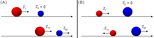
If m1 > m2, the final speed of ball 1 will be positive, v1f > 0, since m1 − m2 > 0, the final speed of ball 2 will also be positive, v2f > 0. This means that after the collision, ball 1 continues to move in the same direction of the trajectory with a lower speed, and ball 2, which was at rest, begins to move in the same direction (Figure 2-A).
If m1 < m2, the final speed of ball 1 will be negative, v1f < 0, since m1 − m2 < 0, the final speed of ball 2 will be positive, v2f > 0. This means that ball 1 moveing in the same direction of the trajectory, reverses its movement after the impact and returns in the oposite direction the trajectory, ball 2 begins to move in the same direction of the trajectory (Figure 2-B).
Substituting solution (XIV) into equation (XII)
\[
\begin{gather}
v_{2f}=\frac{1}{m_{2}}(m_{1}v_{1}-m_{1}v_{1})\\[5pt]
v_{2f}=0 \tag{XV}
\end{gather}
\]
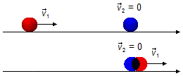
Note: Solutions (XIV) and (XV) were not used, as they are physically impossible.
Ball 1 would continue with its speed in the same direction of the trajectory and ball 2 would
continue at rest, there would be no collision, ball 1 would be a “ghost ball” passing through
ball 2 (Figure 3).
b) Lettng m1 = m2 = m in system (XI)
\[
\begin{gather}
\left\{
\begin{matrix}
\;\cancel{m}v_{1}-\cancel{m}v_{2}=\cancel{m}v_{1f}+\cancel{m}v_{2f}\\
\;\cancel{m}v_{1}^{2}+\cancel{m}v_{2}^{2}=\cancel{m}v_{1f}^{2}+\cancel{m}v_{2f}^{2}
\end{matrix}
\right.
\\[5pt]
\left\{
\begin{matrix}
\;v_{1}-v_{2}=v_{1f}+v_{2f}\\
\;v_{1}^{2}+v_{2}^{2}=v_{1f}^{2}+v_{2f}^{2}
\end{matrix}
\right.
\end{gather}
\]
solving the first equation for v2f
\[
\begin{gather}
v_{2f}=v_{1}-v_{2}-v_{1f} \tag{XVI}
\end{gather}
\]
and substituting in the second equation
\[
\begin{gather}
v_{1}^{2}+v_{2}^{2}=v_{1f}^{2}+(v_{1}-v_{2}-v_{1f})^{2}
\end{gather}
\]
the term in parentheses on the right-hand side of the equality is of type
\( (a-b-c)^{2}=a^{2}+b^{2}+c^{2}-2ab-2ac+2bc \)
\( (a-b-c)^{2}=a^{2}+b^{2}+c^{2}-2ab-2ac+2bc \)
applying to the equation above
\[
\begin{gather}
v_{1}^{2}+v_{2}^{2}=v_{1f}^{2}+v_{1}^{2}-2v_{1}v_{2}-2v_{1}v_{1f}+v_{2}^{2}+2v_{2}v_{1f}+v_{1f}^{2}
\end{gather}
\]
Note: We can directly multiply the two terms
\[
\begin{array}{l}
\begin{array}{l}
v_{1}-v_{2}-v_{1f}\\
v_{1}-v_{2}-v_{1f}
\end{array}\\
\hline
\begin{alignat}{4}
& v_{1}^{2} & - & v_{1}v_{2} & - & v_{1}v_{1f}\\
& & - & v_{1}v_{2} & & & + & v_{2}^{2} & + & v_{2}v_{1f}\\
& & & & - & v_{1}v_{1f} & & & + & v_{2}v_{1f} & + & v_{1f}^{2}\\
\hline
& v_{1}^{2} & - & 2 v_{1}v_{2} & - & 2 v_{1}v_{1f} & + & v_{2}^{2} & + & 2 v_{2}v_{1f} & + & v_{1f}^{2}
\end{alignat}\\
\end{array}
\]
\[
\begin{gather}
\cancel{v_{1}^{2}}+\cancel{v_{2}^{2}}=\cancel{v_{1}^{2}}-2v_{1}v_{2}-2v_{1}v_{1f}+\cancel{v_{2}^{2}}+2v_{2}v_{1f}+v_{1f}^{2}\\[5pt]
0=v_{1f}^{\;2}-2v_{1}v_{2}-2v_{1}v_{1f}+2v_{2}v_{1f}+v_{1f}^{2}\\[5pt]
2v_{1f}^{;2}+\left(2v_{2}-2v_{1}\right)v_{1f}-2v_{1}v_{2}=0
\end{gather}
\]
This is a Quadratuc Equation of type
\( ax^{2}+bx+c=0 \)
where the unknown is the value v1f.
Solution of
\( \underbrace{2}_{a}\underbrace{v_{1f}^{2}}_{x^{2}}+\underbrace{\left(2v_{2}-2v_{1}\right)}_{b}\underbrace{v_{1f}}_{x}-\underbrace{2v_{1}v_{2}}_{c}=0 \)
\( \underbrace{2}_{a}\underbrace{v_{1f}^{2}}_{x^{2}}+\underbrace{\left(2v_{2}-2v_{1}\right)}_{b}\underbrace{v_{1f}}_{x}-\underbrace{2v_{1}v_{2}}_{c}=0 \)
\[
\begin{align}
& \Delta=b^{2}-4ac=\left(2v_{2}-2v_{1}\right)^{2}-4.2\left(-2v_{1}v_{2}\;\right)\\[5pt]
& \Delta=4v_{2}^{2}-8v_{1}v_{2}+4v_{1}^{2}-8\left(-2v_{1}v_{2}\right)\\[5pt]
& \Delta =4v_{1}^{2}-8v_{1}v_{2}+4v_{2}^{2}+16v_{1}v_{2}\\[5pt]
& \Delta=4v_{1}^{2}+8v_{1}v_{2}+4v_{2}^{2}\\[5pt]
& \Delta=4\left(v_{1}^{2}+2v_{1}v_{2}+v_{2}^{2}\right)
\end{align}
\]
the term in parentheses is a special binomia of the type
\( (a^{2}+2ab+b^{2})=(a+b)^{2} \)
\[
\begin{align}
& \Delta =4\left(v_{1}+v_{2}\right)^{2} \\[10pt]
& v_{1f}=\frac{-b\pm \sqrt{\Delta}}{2a}=\frac{-\left(2v_{2}-2v_{1}\right)\pm \sqrt{4\left(v_{1}+v_{2}\right)^{2}}}{2\times 2}\\[5pt]
& v_{1f}=\frac{\cancel{2}\left(v_{1}-v_{2}\right)\pm \cancel{2}\left(v_{1}+v_{2}\right)}{\cancel{2}\times 2}\\[5pt]
& v_{1f}=\frac{v_{1}-v_{2}+v_{1}+v_{2}}{2}\qquad \text{ou}\qquad v_{1f}=\frac{v_{1}-v_{2}-v_{1}-v_{2}}{2}\\[5pt]
& v_{1f}=\frac{2}{2}v_{\;1}\qquad \text{ou}\qquad v_{1f}=-\frac{2}{2}v_{\;2}
\end{align}
\]
\[
\begin{gather}
v_{1f}=v_{1} \tag{XVII}
\end{gather}
\]
\[
\text{or}
\]
\[
\begin{gather}
\bbox[#FFCCCC,10px]
{v_{1f}=-v_{2}}
\end{gather}
\]
substituting this solution into equation (XVI)
\[
\begin{gather}
v_{2f}=v_{1}-v_{2}-(-v_{2})\\[5pt]
v_{2f}=v_{1}-v_{2}+v_{2}
\end{gather}
\]
\[
\begin{gather}
\bbox[#FFCCCC,10px]
{v_{2f}=v_{1}}
\end{gather}
\]
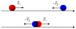
In this case, the balls change their speed, ball 1 returns in the oposite direction of the trajectory
with the speed equal to the speed of ball 2, while ball 2 returns in the same direction of the
trajectory with the speed equal to the speed of ball 1 (Figure 4).

Substituting the solution (XVII) into equation (XVI)
\[
\begin{gather}
v_{2f}=v_{1}-v_{2}-v_{1}\\[5pt]
v_{2f}=-v_{2} \tag{XVIII}
\end{gather}
\]
Note: Solutions (XVII) and (XVIII) were not used, as they are physically impossible.
Ball 1 would continue with its speed in the same direction of the trajectory and ball 2 would
continue with its speed in the oposite direction of the trajectory, there would be no collision,
there would be two “ghost balls” passing through each other (Figure 5).
advertisement

Fisicaexe - Physics Solved Problems by Elcio Brandani Mondadori is licensed under a Creative Commons Attribution-NonCommercial-ShareAlike 4.0 International License .