Exercício Resolvido de Massa e Quantidade de Movimento
publicidade
Calcular por integração direta o vetor centro de massa da placa triangular, de massa M e densidade
constante, indicada na figura.
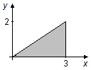
Esquema do problema:
A hipotenusa passa pelos pontos (0. 0) e (3, 2), a equação da reta tem a forma
\[ \bbox[#99CCFF,10px]
{y=ax+b}
\]
substituindo os pontos nesta equação encontramos os coeficientes a e b
\[
\left\{
\begin{matrix}
\;0=a.0+b\\
\;2=a.3+b
\end{matrix}
\right.
\]
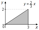
Figura 1
da primeira equação, temos imediatamente que b = 0, substituindo este valor na segunda equação
\[
\begin{gather}
2=3a+0\\
a=\frac{2}{3}
\end{gather}
\]
portanto, a equação da reta será
\[
\begin{gather}
y=\frac{2}{3}x \tag{I}
\end{gather}
\]
Solução
O vetor centro de massa é dado por
\[
\begin{gather}
\bbox[#99CCFF,10px]
{{\mathbf{r}}_{C.M.}=\frac{1}{M}\int{\mathbf{r}}\;dm} \tag{II}
\end{gather}
\]
O vetor posição (r) é dado por
\[
\begin{gather}
\mathbf{r}=x\;\mathbf{i}+y\;\mathbf{j} \tag{III}
\end{gather}
\]
o elemento de massa (dm) pode ser obtido pela densidade superficial de massa
\[ \bbox[#99CCFF,10px]
{\sigma =\frac{dm}{da}}
\]
\[
\begin{gather}
dm=\sigma \;da \tag{IV}
\end{gather}
\]
substituindo as expressões (III) e (IV) na expressão (II)
\[
\begin{gather}
{\mathbf{r}}_{C.M.}=\frac{1}{M}\int\left(x\;\mathbf{i}+y\;\mathbf{j}\right)\sigma\;da \tag{V}
\end{gather}
\]
o elemento de área, em coordenadas cartesianas, será
\[
\begin{gather}
da=dx\;dy \tag{VI}
\end{gather}
\]
substituindo a expressão (VI) na expressão (V)
\[
{\mathbf{r}}_{C.M.}=\frac{1}{M}\int \int\left(x\;\mathbf{i}+y\;\mathbf{j}\right)\sigma\;dx\;dy
\]
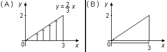
A densidade σ é constante e, portanto ela “sai” da integral. Os limites de integração serão, integrando
primeiro em y, dy varia de 0 até a reta
\( y=\frac{2}{3}x \)
(Figura 2-A), integrando em x, dx varia de 0 até 3 (Figura 2-B).
\[
{\mathbf{r}}_{C.M.}=\frac{\sigma}{M}\int_{0}^{3}\int_{0}^{{\frac{2}{3}x}}\left(x\;\mathbf{i}+y\;\mathbf{j}\right)\;dy\;dx
\]
como a integral da soma é a soma das integrais
\[
\begin{gather}
{\mathbf{r}}_{C.M.}=\frac{\sigma}{M}\left[\int_{0}^{3}\int_{0}^{{\frac{2}{3}x}}x\;dy\;dx\;\mathbf{i}+\int_{0}^{3}\int_{0}^{{\frac{2}{3}x}}y\;dy\;dx\;\mathbf{j}\right]\\[5pt]
{\mathbf{r}}_{C.M.}=\frac{\sigma}{M}\left[\int_{0}^{3}x\left(\int_{0}^{{\frac{2}{3}x}}dy\right)\;dx\;\mathbf{i}+\int_{0}^{3}\left(\int_{0}^{{\frac{2}{3}x}}y\;dy\right)\;dx\;\mathbf{j}\right]
\end{gather}
\]
como y é função de x
\( \left(y=f(x)=\frac{2}{3}x\right) \),
integramos primeiro em y até a função f(x) e depois em x entre os extremos numéricos.
Integração de \( \displaystyle \int_{0}^{{\frac{2}{3}x}}dy \)
\[
\int_{0}^{{\frac{2}{3}x}}dy\Rightarrow\left.y\;\right|_{\;0}^{\;\frac{2}{3}x}\Rightarrow\frac{2}{3}x-0\Rightarrow \frac{2}{3}x
\]
Integração de \( \displaystyle \int_{0}^{{\frac{2}{3}x}}y\;dy \)
\[
\int_{0}^{{\frac{2}{3}x}}y\;dy\Rightarrow\left.\frac{y^{1+1}}{1+1}\;\right|_{\;0}^{\;\frac{2}{3}x}\Rightarrow\left.\frac{y^{\;2}}{2}\;\right|_{\;0}^{\;\frac{2}{3}x}\Rightarrow\frac{1}{2}\left[\left(\frac{2}{3}x\right)^{2}-0^{2}\right]\Rightarrow\frac{1}{2}.\frac{4}{9}x^{2}\Rightarrow \frac{2}{9}x^{2}
\]
\[
\begin{gather}
{\mathbf{r}}_{C.M.}=\frac{\sigma}{M}\left[\int_{0}^{3}x\left(\frac{2}{3}x\right)\;dx\;\mathbf{i}+\int_{0}^{3}\left(\frac{2}{9}x^{2}\right)\;dx\;\mathbf{j}\right]\\[5pt]
{\mathbf{r}}_{C.M.}=\frac{\sigma}{M}\left[\int_{0}^{3}{\frac{2}{3}}x^{2}\;dx\;\mathbf{i}+\int_{0}^{3}{\frac{2}{9}}x^{2}\;dx\;\mathbf{j}\right]\\[5pt]
{\mathbf{r}}_{C.M.}=\frac{\sigma}{M}\left[\frac{2}{3}\int_{0}^{3}x^{2}\;dx\;\mathbf{i}+\frac{2}{9}\int_{0}^{3}x^{2}\;dx\;\mathbf{j}\right]
\end{gather}
\]
Integração de \( \displaystyle \int_{0}^{3}x^{2}\;dx \)
\[
\int_{0}^{3}x^{2}\;dx\Rightarrow\left.\frac{x^{2+1}}{2+1}\;\right|_{\;0}^{\;\frac{2}{3}x}\Rightarrow\left.\frac{x^{3}}{3}\;\right|_{\;0}^{\;\frac{2}{3}x}\Rightarrow\frac{1}{3}\left(3^{3}-0^{3}\right)\Rightarrow \frac{27}{3}\Rightarrow{9}
\]
\[
\begin{gather}
{\mathbf{r}}_{C.M.}=\frac{\sigma}{M}\left[\frac{2}{3}.9\;\mathbf{i}+\frac{2}{9}.9\;\mathbf{j}\right]\\
{\mathbf{r}}_{C.M.}=\frac{\sigma}{M}\left[6\;\mathbf{i}+2\;\mathbf{j}\right] \tag{VII}
\end{gather}
\]
A densidade superficial de um corpo é dada por
\[
\begin{gather}
\bbox[#99CCFF,10px]
{\sigma =\frac{M}{A}} \tag{VIII}
\end{gather}
\]
substituindo a expressão(VIII) na expressão (VII)
\[
\begin{gather}
{\mathbf{r}}_{C.M.}=\frac{1}{\cancel{M}}\frac{\cancel{M}}{A}\left[6\;\mathbf{i}+2\;\mathbf{j}\right]\\
{\mathbf{r}}_{C.M.}=\frac{1}{A}\left[6\;\mathbf{i}+2\;\mathbf{j}\right] \tag{IX}
\end{gather}
\]
onde A é a área do corpo, a área de um triângulo é dada por
\[ \bbox[#99CCFF,10px]
{A=\frac{bh}{2}}
\]
para b = 3 e h =2, a área será
\[
\begin{gather}
A=\frac{3.2}{2}\\
A=3 x \tag{X}
\end{gather}
\]
substituindo o resultado (X) em (IX)
\[
\begin{gather}
{\mathbf{r}}_{C.M.}=\frac{1}{3}.\left[6\;\mathbf{i}+2\;\mathbf{j}\right]\\
{\mathbf{r}}_{C.M.}=\frac{6}{3}\;\mathbf{i}+\frac{2}{3}\;\mathbf{j}
\end{gather}
\]
\[ \bbox[#FFCCCC,10px]
{{\mathbf{r}}_{C.M.}=2\;\mathbf{i}+\frac{2}{3}\;\mathbf{j}}
\]
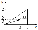
Figura 3
Observação: Alternativamente poderíamos integrar primeiro em x e depois em y,
invertendo a ordem de integração (isto é garantido pelo Teorema de Fubini). Para isto devemos inverter
a expressão (I), escrevendo x em função de y,
\( x=f(y)=\frac{3}{2}y \).
Os limites de integração serão, integrando primeiro em x, dx varia da reta \( x=\frac{3}{2}y \) até a reta x = 3 (Figura 4-A). Integrando depois em y, dy varia de 0 até 2 (Figura 4-B).
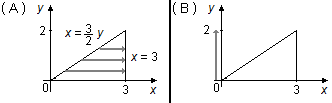 Figura 4
Os limites de integração serão, integrando primeiro em x, dx varia da reta \( x=\frac{3}{2}y \) até a reta x = 3 (Figura 4-A). Integrando depois em y, dy varia de 0 até 2 (Figura 4-B).
\[
{\mathbf{r}}_{C.M.}=\frac{\sigma }{M}\int_{0}^{2}\int_{{\frac{3}{2}y}}^{3}\left(x\;\mathbf{i}+y\;\mathbf{j}\right)\;dx\;dy
\]
isto nos leva as integrais
\[
{\mathbf{r}}_{C.M.}=\frac{\sigma}{M}\;\left[\int_{0}^{2}\left(\int_{{\frac{3}{2}y}}^{3}x\;dx\right)\;dy\;\mathbf{i}+\int_{0}^{2}y\left(\int_{{\frac{3}{2}y}}^{3}\;dx\right)\;dy\;\mathbf{j}\right]
\]
o que nos leva ao mesmo resultado
\[
{\mathbf{r}}_{C.M.}=2\;\mathbf{i}+\frac{2}{3}\;\mathbf{j}
\]
publicidade

Fisicaexe - Exercícios Resolvidos de Física de Elcio Brandani Mondadori está licenciado com uma Licença Creative Commons - Atribuição-NãoComercial-Compartilha Igual 4.0 Internacional .