Um fio de comprimento L é carregado com uma carga Q distribuída uniformemente pelo fio,
determinar:
a) O potencial elétrico num ponto P da reta que contém o fio, x > L (coordenada do
ponto P externa ao fio);
b) O vetor campo elétrico no mesmo ponto.
Dados do problema:
- Comprimento do fio: L;
- Carga do fio: Q.
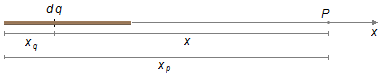
Esquema do problema:
Adotando como referencial a ponta esquerda do fio, a distância da origem ao ponto P é igual
xp, a distância da origem a um elemento de carga dq é igual a xq
a distância de um elemento de carga dq ao ponto P será x (Figura 1).
Solução:
a) O potencial elétrico é dado por
\[
\begin{gather}
\bbox[#99CCFF,10px]
{V=\frac{1}{4\pi\epsilon_0}\int{\frac{d q}{r}}} \tag{I}
\end{gather}
\]
Com r=x, a distância de um elemento de carga ao ponto onde se deseja calcular o potencial
elétrico será (Figura 1)
\[
\begin{gather}
x=x_p-x_q \tag{II}
\end{gather}
\]
Da equação da densidade linear de carga λ obtemos o elemento de carga dq
\[
\begin{gather}
\bbox[#99CCFF,10px]
{\lambda=\frac{d q}{d s}}
\end{gather}
\]
\[
\begin{gather}
dq=\lambda\;ds \tag{III}
\end{gather}
\]
onde ds é um elemento de comprimento do fio
\[
\begin{gather}
ds=dx_q \tag{IV}
\end{gather}
\]
substituindo a equação (IV) na equação (III)
\[
\begin{gather}
dq=\lambda\;dx_q \tag{V}
\end{gather}
\]
substituindo as equações (II) e (V) na equação (I)
\[
\begin{gather}
V=\frac{1}{4\pi\epsilon_0}\int{\frac{\lambda dx_q}{(x_p-x_q)}} \tag{VI}
\end{gather}
\]
Como a densidade de carga λ é constante, a integral depende apenas de xq,
ela pode “sair” da integral, podemos escrever
\[
\begin{gather}
V=\frac{\lambda}{4\pi\epsilon_0}\int{\frac{dx_q}{(x_p-x_q)}}
\end{gather}
\]
Os limites de integração serão 0 e L (o comprimento do fio carregado)
\[
\begin{gather}
V=\frac{\lambda}{4\pi\epsilon_0}\int_0^L{\frac{dx_q}{(x_p-x_q)}}
\end{gather}
\]
Integral de
\( \displaystyle \int_0^L{\frac{dx_q}{(x_p-x_q)}} \)
fazendo a mudança de variável
\[
\begin{array}{l}
u=x_p-x_q \\
\dfrac{du}{dx_q}=-1\Rightarrow-dx\Rightarrow dx=-du
\end{array}
\]
fazendo a mudança dos extremos de integração
para
xq=0
temos
\( u=x_p-0\Rightarrow u=x_p \)
para
xq=
L
temos
\( u=x_p-L \)
\[
\begin{align}
\displaystyle \int_{x_p}^{x_p-L}\frac{-du}{u} & \Rightarrow\displaystyle -\int_{x_p}^{x_p-L}{\frac{1}{u}du}\Rightarrow -\;\left.\ln u\;\right|_{\;x_p}^{\;x_p-L}\Rightarrow \\
& \Rightarrow-\left[\ln (x_p-L)-\ln x_p\right]\Rightarrow \\
& \Rightarrow\ln x_p-\ln (x_p-L)\Rightarrow \ln\left(\dfrac{x_p}{x_p-L}\right)
\end{align}
\]
\[
\begin{gather}
V=\frac{\lambda}{4\pi\epsilon_0}\ln \left(\frac{x_p}{x_p-L}\right) \tag{VII}
\end{gather}
\]
A densidade linear de carga pode ser escrita
\[
\begin{gather}
\lambda=\frac{Q}{L} \tag{VIII}
\end{gather}
\]
substituindo a equação (VIII) na equação (VII)
\[
\begin{gather}
\bbox[#FFCCCC,10px]
{V=\frac{Q}{4\pi\epsilon_0L}\ln \left(\frac{x_p}{x_p-L}\right)}
\end{gather}
\]
b) O vetor campo elétrico é dado por
\[
\begin{gather}
\bbox[#99CCFF,10px]
{\mathbf E=-\nabla V}
\end{gather}
\]
onde
\( \nabla \)
é o operador nabla dado por
\( \left(\dfrac{\partial}{\partial x}\;\mathbf i+\dfrac{\partial}{\partial y}\;\mathbf j+\dfrac{\partial}{\partial z}\;\mathbf k\right) \)
\[
\begin{gather}
\mathbf E=-\left(\frac{\partial}{\partial x}\;\mathbf i+\frac{\partial}{\partial y}\;\mathbf j+\frac{\partial}{\partial z}\;\mathbf k\right)V\\
\mathbf E=-\left(\frac{\partial V}{\partial x}\;\mathbf i+\frac{\partial V}{\partial y}\;\mathbf j+\frac{\partial V}{\partial z}\;\mathbf k\right)
\end{gather}
\]
O problema é unidimensional, portanto as derivadas em y e z são nulas.
Derivada parcial do potencial em relação a
x
\[
\begin{gather}
\frac{dV}{dx_p}=\frac{d}{dx_p}\frac{Q}{4\pi\epsilon_0L}\ln\left(\frac{x_p}{x_p-L}\right)
\end{gather}
\]
o termo
\( \frac{Q}{4\pi\epsilon_0L} \)
é constante, portanto pode “sair” da derivada
\[
\begin{gather}
\frac{dV}{dx_p}=\frac{Q}{4\pi\epsilon_0L}\frac{d}{dx_p}\ln\left(\frac{x_p}{x_p-L}\right)
\end{gather}
\]
a função
V(
xp) é uma função composta cuja derivada é dada pela regra da cadeia
\[
\begin{gather}
\frac{dV[u(x_p)]}{dx_p}=\frac{dV}{du}\frac{du}{dx_p}
\end{gather}
\]
com
\( V(u)=\ln u \)
e
\( u(x_p)=\frac{x_p}{x_p-L} \),
assim as derivadas serão
\[
\begin{gather}
\frac{dV(u)}{du}=\frac{1}{u}
\end{gather}
\]
a função
u(
xp) é um quociente de funções (em
xp),
\( u=\frac{f}{g} \),
a derivada é da forma
\( u'=\frac{f'g-g'f}{g^2} \),
com
f =
xp e
g =
xp−
L
\[
\begin{align}
\frac{du(x_p)}{dx_p} & =\frac{1\times(x_p-L)-x_p\times 1}{(x_p-L)^2}\Rightarrow\frac{(x_p-L)-x_p}{(x_p-L)^2}\Rightarrow \\
& \Rightarrow\frac{x_p-L-x_p}{(x_p-L)^2}\Rightarrow \frac{-L}{(x_p-L)^2}
\end{align}
\]
Substituindo as derivadas
\[
\begin{gather}
\frac{dV}{dx_p}=\frac{Q}{4\pi\epsilon_0\cancel{L}}\frac{1}{ \left[ \dfrac{x_p}{\cancel{x_p-L}} \right] }\left[-\frac{\cancel{L}}{(x_p-L)^{\cancel 2}}\right] \\[5pt]
\frac{dV}{dx_p}=-{\frac{Q}{4\pi\epsilon_0}}\frac{1}{x_p(x_p-L)}
\end{gather}
\]
\[
\begin{gather}
\mathbf E=-\left[-\frac{Q}{4\pi\epsilon_0 L}\left(\frac{L}{x_p(x_p-L)}\right)\right]\mathbf i
\end{gather}
\]
\[
\begin{gather}
\bbox[#FFCCCC,10px]
{\mathbf E=\frac{1}{4\pi\epsilon_0} \frac{Q}{x_p(x_p-L)}\mathbf i}
\end{gather}
\]
e o módulo do campo elétrico será
\[
\begin{gather}
\bbox[#FFCCCC,10px]
{E=\frac{1}{4\pi\epsilon_0}\frac{Q}{x_p(x_p-L)}}
\end{gather}
\]