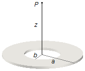
Um disco de raio a possui no centro um orifício de raio b e está carregado uniformemente
com uma carga Q. Calcule o vetor campo elétrico num ponto P sobre o eixo de simetria
perpendicular ao plano do disco a uma distância z do seu centro.
Dados do problema:
- Raio do disco: a;
- Raio do orifício: b;
- Carga do disco: Q;
- Distância ao ponto onde se quer o campo elétrico: z.
Esquema do problema:
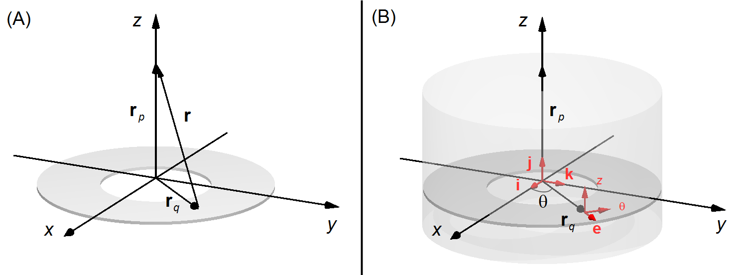
O vetor posição r vai de um elemento de carga do disco dq até o ponto P onde se deseja
calcular o campo elétrico, o vetor rq localiza o elemento de carga em relação à
origem do referencial e o vetor rp localiza o ponto P (Figura 1-A).
\[
\begin{gather}
\mathbf r={\mathbf r}_p-{\mathbf r}_q
\end{gather}
\]
Pela geometria do problema devemos escolher coordenadas cilíndricas (Figura 1-B), o vetor
rq, só possui componente na direção er,
\( {\mathbf r}_q=r_q\;\mathbf{e}_{r} \),
e o vetor rp só possui componente na direção ez,
\( {\mathbf r}_p=r_p\;\mathbf{e}_{z} \).
Fazendo a conversão de coordenadas cilíndricas para coordenadas cartesianas x, y e
z são dados por
\[
\begin{gather}
\left\{
\begin{array}{l}
x=r_q\cos\theta \\
y=r_q\operatorname{sen}\theta \\
z=z
\end{array}
\right. \tag{I}
\end{gather}
\]
Observação: Na Figura 1-B, i, j e k são os vetores unitários da base do
sistema de coordenadas cartesianas, e er, eθ e
ez são os vetores unitários da base do sistema de coordenadas cilíndricas.
Depois da conversão o vetor rq, é escrito como
\( {\mathbf r}_q=x\;\mathbf i+y\;\mathbf j \),
e o vetor rp como
\( {\mathbf r}_p=z\;\mathbf k \).
O vetor posição será
\[
\begin{gather}
\mathbf r=z\;\mathbf k-\left(x\;\mathbf i+y\;\mathbf j\right) \\[5pt]
\mathbf r=-x\;\mathbf i-y\;\mathbf j+z\;\mathbf k \tag{II}
\end{gather}
\]
Da equação (II) o módulo do vetor posição r será
\[
\begin{gather}
r^2=(-x)^2+(-y)^2+z^2\\[5pt]
r=\left(x^2+y^2+z^2\right)^{\frac{1}{2}} \tag{III}
\end{gather}
\]
Solução:
O vetor campo elétrico é dado por
\[
\begin{gather}
\bbox[#99CCFF,10px]
{\mathbf E=\frac{1}{4\pi\epsilon_0}\int{\frac{dq}{r^2}\;\frac{\mathbf r}{r}}}
\end{gather}
\]
\[
\begin{gather}
\mathbf E=\frac{1}{4\pi\epsilon_0}\int{\frac{dq}{r^{3}}\;\mathbf r} \tag{IV}
\end{gather}
\]
Da equação da densidade superficial de carga σ obtemos o elemento de carga dq
\[
\begin{gather}
\bbox[#99CCFF,10px]
{\sigma=\frac{dq}{dA}}
\end{gather}
\]
\[
\begin{gather}
dq=\sigma\;dA \tag{V}
\end{gather}
\]
onde dA é um elemento de área.
O elemento de área em coordenadas cartesianas é
\[
\begin{gather}
dA=dx\;dy
\end{gather}
\]
para obter o elemento de área em coordenadas polares calculamos o Jacobiano dado pelo determinante
\[
\begin{gather}
J=\left|
\begin{matrix}
\;\dfrac{\partial x}{\partial r} &\dfrac{\partial x}{\partial \theta }\;\\
\;\dfrac{\partial y}{\partial r} &\dfrac{\partial y}{\partial \theta }\;
\end{matrix}\right|
\end{gather}
\]
Cálculo das derivadas parciais das funções
x e
y dadas em (III)
\( x=r_q\cos\theta \):
\( \dfrac{\partial x}{\partial r_q}=\dfrac{\partial (r_q\cos\theta\;)}{\partial r_q}=\cos\theta \dfrac{\partial r_q}{\partial r_q}=\cos\theta .1=\cos\theta \text{, } \)
\[ \dfrac{\partial x}{\partial r_q}=\dfrac{\partial (r_q\cos\theta\;)}{\partial r_q}=\cos\theta \dfrac{\partial r_q}{\partial r_q}=\cos\theta .1=\cos\theta \]
na derivada em
rq o valor de θ é constante e o cosseno sai da
derivada.
\( \dfrac{\partial x}{\partial \theta }=\dfrac{\partial (r_q\cos\theta)}{\partial \theta }=r_q\dfrac{\partial (\cos\theta )}{\partial\theta }=r_q(-\operatorname{sen}\theta)=-r_q\operatorname{sen}\theta \text{, } \)
\[ \dfrac{\partial x}{\partial \theta }=\dfrac{\partial (r_q\cos\theta)}{\partial \theta }=r_q\dfrac{\partial (\cos\theta )}{\partial\theta }=r_q(-\operatorname{sen}\theta)=-r_q\operatorname{sen}\theta \]
na derivada em θ o valor de
rq é constante e sai da derivada.
\( y=r_q\operatorname{sen}\theta \):
\( \dfrac{\partial y}{\partial r_q}=\dfrac{\partial(r_q\operatorname{sen}\theta )}{\partial r_q}=\operatorname{sen}\theta \dfrac{\partial r_q}{\partial r_q}=\operatorname{sen}\theta .1=\operatorname{sen}\theta \text{, } \)
\[ \dfrac{\partial y}{\partial r_q}=\dfrac{\partial(r_q\operatorname{sen}\theta )}{\partial r_q}=\operatorname{sen}\theta \dfrac{\partial r_q}{\partial r_q}=\operatorname{sen}\theta .1=\operatorname{sen}\theta \]
na derivada em
r o valor de θ é constante e o seno sai da derivada.
\( \dfrac{\partial y}{\partial \theta }=\dfrac{\partial(r_q\operatorname{sen}\theta )}{\partial \theta }=r_q\dfrac{\partial(\operatorname{sen}\theta )}{\partial \theta }=r_q\cos\theta \text{, } \)
\[ \dfrac{\partial y}{\partial \theta }=\dfrac{\partial(r_q\operatorname{sen}\theta )}{\partial \theta }=r_q\dfrac{\partial(\operatorname{sen}\theta )}{\partial \theta }=r_q\cos\theta \]
na derivada em θ o valor de
rq é constante e sai da derivada.
\[
\begin{gather}
dA=dx\;dy=J\;dr_q\;d\theta
\end{gather}
\]
\[
\begin{gather}
J=\left|
\begin{matrix}
\;\cos\theta & -r_q\operatorname{sen}\theta \;\\
\;\operatorname{sen}\theta & r_q\cos\theta
\end{matrix}\right|\\[5pt]
J=\cos\theta\times r_q\cos\theta-(-r_q\operatorname{sen}\theta\times\operatorname{sen}\theta)\\[5pt]
J=r_q\cos^2\theta +r_q\operatorname{sen}^2\theta\\[5pt]
J=r_q(\underbrace{\cos^2\theta +\operatorname{sen}^{\;2}\theta}_1)\\[5pt]
J=r_q
\end{gather}
\]
\[
\begin{gather}
dA=r_q\;dr_q\;d\theta \tag{VI}
\end{gather}
\]
substituindo a equação (VI) na equação (V)
\[
\begin{gather}
dq=\sigma r_q\;dr_q\;d\theta \tag{VII}
\end{gather}
\]
Substituindo as equações (II), (II) e (VII) na equação (IV), e como a integração é feita sobre a
superfície do disco, depende de duas variáveis rq e θ, temos uma integral dupla
\[
\begin{gather}
\mathbf E=\frac{1}{4\pi\epsilon_0}\iint {\frac{\sigma r_q\;dr_q\;d\theta}{\left[\left(x^2+y^2+z^2\right)^{\frac{1}{2}}\right]^{3}}}\left(-x\;\mathbf i-y\;\mathbf j+z\;\mathbf k\right)\\[5pt]
\mathbf E=\frac{1}{4\pi\epsilon_0}\iint {\frac{\sigma r_q\;dr_q\;d\theta}{\left(x^2+y^2+z^2\right)^{\frac{3}{2}}}}\left(-x\;\mathbf i-y\;\mathbf j+z\;\mathbf k\right) \tag{VIII}
\end{gather}
\]
substituindo as equações de (I) na equação (VIII)
\[
\begin{gather}
\mathbf E=\frac{1}{4\pi\epsilon_0}\iint {\frac{\sigma r_q\;dr_q\;d\theta}{\left[\left(r_q\cos\theta\right)^2+\left(r_q\operatorname{sen}\theta\right)^2+z^2\right]^{\frac{3}{2}}}\left(-r_q\cos\theta\;\mathbf i-r_q\operatorname{sen}\theta\;\mathbf j+z\mathbf k\right)}\\[5pt]
\mathbf E=\frac{1}{4\pi\epsilon_0}\iint {\frac{\sigma r_q\;dr_q\;d\theta}{\left[r_q^2\cos^{\;2}\theta+r_q^2\operatorname{sen}^2\theta+z^2\;\right]^{\frac{3}{2}}}\left(-r_q\cos\theta\;\mathbf i-r_q\operatorname{sen}\theta\;\mathbf j+z\;\mathbf k\right)}\\[5pt]
\mathbf E=\frac{1}{4\pi\epsilon_0}\iint {\frac{\sigma r_q\;dr_q\;d\theta}{\left[r_q^2\underbrace{\left(\cos^2\theta+\operatorname{sen}^2\theta\right)}_1+z^2\right]^{\frac{3}{2}}}\left(-r_q\cos\theta\;\mathbf i-r_q\operatorname{sen}\theta\;\mathbf j+z\;\mathbf k\right)}\\[5pt]
\mathbf E=\frac{1}{4\pi\epsilon_0}\iint {\frac{\sigma r_q\;dr_q\;d\theta}{\left(r_q^2+z^2\right)^{\frac{3}{2}}}\left(-r_q\cos\theta\;\mathbf i-r_q\operatorname{sen}\theta\;\mathbf j+z\;\mathbf k\right)}
\end{gather}
\]
A densidade de carga σ é constante ela pode “sair” da integral, e a integral da soma é igual à soma
das integrais
\[
\begin{gather}
\mathbf E=\frac{\sigma}{4\pi\epsilon_0}\left(-\iint {\frac{r_q^2\cos\theta \;dr_q\;d\theta}{\left(r_q^2+z^2\right)^{\frac{3}{2}}}}\;\mathbf i-\iint {\frac{r_q^2\operatorname{sen}\theta \;dr_q\;d\theta}{\left(r_q^2+z^2\right)^{\frac{3}{2}}}}\;\mathbf j+z\iint {\frac{r_q\;dr_q\;d\theta}{\left(r_q^2+z^2\right)^{\frac{3}{2}}}}\;\mathbf k\right)
\end{gather}
\]
Os limites de integração serão de b a a em drq, ao longo do raio do disco,
e de 0 e 2π em dq, uma volta completa no disco, e como não existem termos “cruzados “ em
r e θ as integrais podem ser separadas
\[
\begin{align}
\mathbf E=&\frac{\sigma}{4\pi\epsilon_0}\left(-\int_{b}^a{\frac{r_q^2\;dr_q}{\left(r_q^2+z^2\right)^{\frac{3}{2}}}}\underbrace{\int_0^{{2\pi}}{\cos\theta \;d\theta}}_0\;\mathbf i-\int_{b}^a{\frac{r_q^2\;dr_q}{\left(r_q^2+z^2\right)^{\frac{3}{2}}}}\underbrace{\int_0^{{2\pi}}{\operatorname{sen}\theta \;d\theta}}_0\;\mathbf j+\right. \\
&\left.+z\int_{b}^a{\frac{r_q\;dr_q}{\left(r_q^2+z^2\right)^{\frac{3}{2}}}}\int_0^{{2\pi}}{d\theta }\;\mathbf k\right)
\end{align}
\]
Integração de
\( \displaystyle \int_0^{{2\pi}}\cos\theta \;d\theta \)
1.º método
\[
\begin{align}
\int_0^{{2\pi}}\cos\theta \;d\theta &=\left.\operatorname{sen}\theta\;\right|_{\;0}^{\;2\pi}=\operatorname{sen}2\pi-\operatorname{sen}0=\\
&=0-0=0
\end{align}
\]
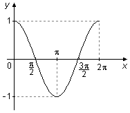
2.º método
O gráfico de cosseno entre 0 e 2π possui uma área “positiva” acima do eixo-x, entre 0 e
\( \frac{\pi}{2} \)
e entre
\( \frac{3\pi}{2} \)
e 2π, e uma área “negativa” abaixo do eixo-x, entre
\( \frac{\pi}{2} \)
e
\( \frac{3\pi}{2} \),
estas duas áreas se cancelam no cálculo da integral, sendo o valor da integral
igual à zero (Figura 2).
Integração de
\( \displaystyle \int_0^{{2\pi}}\operatorname{sen}\theta \;d\theta \)
1.º método
\[
\begin{align}
\int_0^{{2\pi}}\operatorname{sen}\theta \;d\theta &=\left.-\cos\theta \;\right|_{\;0}^{\;2\pi}=-(\cos 2\pi-\cos 0)=\\
&=-(1-1)=0
\end{align}
\]
2.º método
O gráfico do seno entre 0 e 2π possui uma área “positiva” acima do eixo-x, entre 0 e π,
e uma área “negativa” abaixo do eixo-x, entre π e 2π, estas duas áreas se cancelam no
cálculo da integral, sendo o valor da integral zero (Figura 3).
Observação: As duas integrais, nas direções i e j, que são nulas
representam o cálculo matemático para a afirmação que se faz usualmente de que as componentes do campo
elétrico paralelas ao plano-xy dEP se anulam. Apenas as
componentes normais ao plano dEN contribuem para o campo elétrico total
(Figura 4).
Integração de
\( \displaystyle \int_{b}^a{\frac{r_q\;dr_q}{\left(r_q^2+z^2\right)^{\frac{3}{2}}}} \)
fazendo a mudança de variável
\[
\begin{array}{l}
u=r_q^2+z^2\\[5pt]
\dfrac{du}{dr_q}=2r_q\Rightarrow dr_q=\dfrac{du}{2r_q}
\end{array}
\]
fazendo a mudança dos extremos de integração
para
rq =
b
temos
\( u=b^2+z^2 \)
para
rq =
a
temos
\( u=a^2+z^2 \)
\[
\begin{align}
\int_{{b^2+z^2}}^{{a^2+z^2}}{\frac{r_q}{u^{\frac{3}{2}}}\;\frac{du}{2r_q}} &\Rightarrow\frac{1}{2}\int_{{b^2+z^2}}^{{a^2+z^2}}{\frac{1}{u^{\frac{3}{2}}}\;du}\Rightarrow\;\frac{1}{2}\left.\frac{u^{-{\frac{3}{2}+1}}}{-{\frac{3}{2}+1}}\;\right|_{\;b^2+z^2}^{\;a^2+z^2}\Rightarrow\\[5pt]
&\Rightarrow\frac{1}{2}\left.\frac{u^{\frac{-3+2}{2}}}{\frac{-{3+2}}{2}}\;\right|_{\;b^2+z^2}^{\;a^2+z^2}\Rightarrow\frac{1}{2}\left.\frac{u^{-{\frac{1}{2}}}}{-{\frac{1}{2}}}\;\right|_{\;b^2+z^2}^{\;a^2+z^2}\Rightarrow\\[5pt]
&\Rightarrow\left.-u^{-{\frac{1}{2}}}\;\right|_{\;b^2+z^2}^{\;a^2+z^2}\Rightarrow\left.-{\frac{1}{u^{\frac{1}{2}}}}\;\right|_{\;b^2+z^2}^{\;a^2+z^2}\Rightarrow\\[5pt]
&\Rightarrow-\left(\frac{1}{\sqrt{a^2+z^2}}-\frac{1}{\sqrt{\;b^2+z^2}}\right)\Rightarrow\\[5pt]
&\Rightarrow\frac{1}{\sqrt{b^2+z^2\;}}-\frac{1}{\sqrt{\;a^2+z^2\;}}
\end{align}
\]
Integração de
\( \displaystyle \int_0^{{2\pi}}d\theta \)
\[
\begin{gather}
\int_0^{{2\pi}}d\theta =\left.\theta \;\right|_{\;0}^{\;2\pi}=2\pi-0=2\pi
\end{gather}
\]
\[
\begin{gather}
\mathbf E=\frac{\sigma}{4\pi\epsilon_0}\left[0\;\mathbf i-0\;\mathbf j+z\;\left(\frac{1}{\sqrt{b^2+z^2\;}}-\frac{1}{\sqrt{a^2+z^2\;}}\right)2\pi\;\mathbf k\right]\\[5pt]
\mathbf E=\frac{\sigma}{\cancelto{2}{4}\cancel{\pi} \epsilon_0}\left[z\left(\frac{1}{\sqrt{b^2+z^2}}-\frac{1}{\sqrt{a^2+z^2\;}}\right)\cancel{2}\cancel{\pi}\;\mathbf k\right]
\end{gather}
\]
\[
\begin{gather}
\bbox[#FFCCCC,10px]
{\mathbf E=\frac{\sigma z}{2\epsilon_0}\left(\frac{1}{\sqrt{b^2+z^2\;}}-\frac{1}{\sqrt{a^2+z^2}}\;\right)\;\mathbf k}
\end{gather}
\]