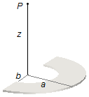
Uma chapa semicircular possui raio externo a e raio interno b. A chapa está carregada com
uma carga total Q distribuída de forma não uniforme diretamente proporcional ao ângulo central
θ do semicírculo de tal forma que
\( 0 \leq \theta \leq \pi \).
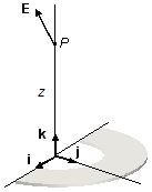
Calcule o vetor campo elétrico num ponto P sobre o eixo perpendicular ao plano do semicírculo que
passa pelo centro de curvatura a uma distância z do seu centro.
Dados do problema:
- Raio externo do semicírculo: a;
- Raio interno do semicírculo: b;
- Carga da chapa: Q;
- Distância ao ponto onde se quer o campo elétrico: z.
Esquema do problema:
A densidade superficial de carga do semicírculo é diretamente proporcional à posição angular da carga
(Figura 1)
\[
\begin{gather}
\sigma(\theta)=\alpha\;\theta \tag{I}
\end{gather}
\]
onde α é uma constante que torna a equação dimensionalmente consistente.
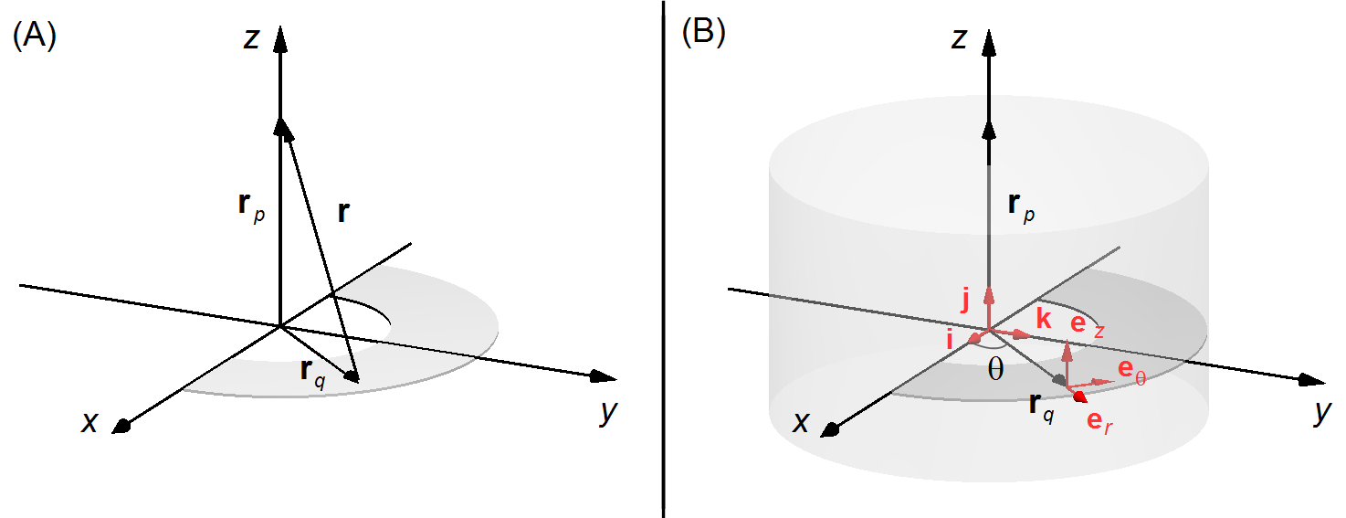
O vetor posição r vai de um elemento de carga dq do disco até o ponto P onde se deseja
calcular o campo elétrico, o vetor rq localiza o elemento de carga em relação à
origem do referencial e o vetor rp localiza o ponto P (Figura 2-A).
\[
\begin{gather}
\mathbf r={\mathbf r}_p-{\mathbf r}_q
\end{gather}
\]
Pela geometria do problema devemos escolher coordenadas cilíndricas (Figura 2-B), o vetor
rq, só possui componente na direção er,
\( {\mathbf r}_q=r_q\;\mathbf e_r \),
e o vetor rp só possui componente na direção ez,
\( {\mathbf r}_p=r_p\;\mathbf e_z \).
Fazendo a conversão de coordenadas cilíndricas para coordenadas cartesianas x, y e
z são dados por
\[
\left\{
\begin{array}{l}
x=r_q\cos\theta \\[5pt]
y=r_q\operatorname{sen}\theta \\[5pt]
z=z
\end{array}
\right. \tag{II}
\]
Observação: Na Figura 2-B, i, j e k são os vetores unitários da base do
sistema de coordenadas cartesianas, e er, eθ e
ez são os vetores unitários da base do sistema de coordenadas cilíndricas.
Depois da conversão o vetor rq, é escrito como
\( {\mathbf r}_q=x\;\mathbf i+y\;\mathbf j \),
e o vetor rp como
\( {\mathbf r}_p=z\;\mathbf k \).
O vetor posição será
\[
\begin{gather}
\mathbf r=z\;\mathbf k-\left(x\;\mathbf i+y\;\mathbf j\right) \\[5pt]
\mathbf r=-x\;\mathbf i-y\;\mathbf j+z\;\mathbf k \tag{III}
\end{gather}
\]
Da equação (III) o módulo do vetor posição r será
\[
\begin{gather}
r^2=(-x)^2+(-y)^2+z^2 \\[5pt]
r=\left(x^2+y^2+z^2\right)^{\frac{1}{2}} \tag{IV}
\end{gather}
\]
Solução:
O vetor campo elétrico é dado por
\[
\begin{gather}
\bbox[#99CCFF,10px]
{\mathbf E=\frac{1}{4\pi\epsilon_0}\int{\frac{dq}{r^2}\;\frac{\mathbf r}{r}}}
\end{gather}
\]
\[
\begin{gather}
\mathbf E=\frac{1}{4\pi\epsilon_0}\int{\frac{dq}{r^3}\;\mathbf r} \tag{V}
\end{gather}
\]
Da equação da densidade superficial de carga σ obtemos o elemento de carga dq
\[
\begin{gather}
\bbox[#99CCFF,10px]
{\sigma=\frac{dq}{dA}}
\end{gather}
\]
\[
\begin{gather}
dq=\sigma(\theta)\;dA \tag{VI}
\end{gather}
\]
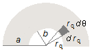
onde dA é um elemento de área de ângulo dθ do disco (Figura 3)
\[
\begin{gather}
dA=r_q\;dr_q\;d\theta \tag{VII}
\end{gather}
\]
substituindo as equações (I) e (VII) na equação (VI)
\[
\begin{gather}
dq=\alpha\theta r_q\;dr_q\;d\theta \tag{VIII}
\end{gather}
\]
Substituindo as equações (III), (IV) e (VIII) na equação (V), e como a integração é feita sobre a
superfície do semicírculo, depende de duas variáveis rq e θ, temos uma integral
dupla
\[
\begin{gather}
\mathbf E=\frac{1}{4\pi\epsilon_0}\iint{\frac{\alpha\theta r_q\;dr_q\;d\theta}{\left[\left(x^2+y^2+z^2\right)^{\frac{1}{2}}\right]^3}}\left(-x\;\mathbf i-y\;\mathbf j+z\;\mathbf k\right) \\[5pt]
\mathbf E=\frac{1}{4\pi\epsilon_0}\iint{\frac{\alpha\theta r_q\;dr_q\;d\theta}{\left(x^2+y^2+z^2\right)^{3/2}}}\left(-x\;\mathbf i-y\;\mathbf j+z\;\mathbf k\right) \tag{IX}
\end{gather}
\]
substituindo as equações (II) na equação (IX)
\[
\begin{gather}
\mathbf E=\frac{1}{4\pi\epsilon_0}\iint{\frac{\alpha\theta r_q\;dr_q\;d\theta}{\left[\left(r_q\cos\theta\right)^2+\left(r_q\operatorname{sen}\theta\right)^2+z^2\right]^{3/2}}\left(-r_q\cos\theta\;\mathbf i-r_q\operatorname{sen}\theta\;\mathbf j+z\;\mathbf k\right)} \\[5pt]
\mathbf E=\frac{1}{4\pi\epsilon_0}\iint{\frac{\alpha\theta r_q\;dr_q\;d\theta}{\left[r_q^2\cos^2\theta+r_q^2\operatorname{sen}^2\theta+z^2\right]^{3/2}}\left(-r_q\cos\theta\;\mathbf i-r_q\operatorname{sen}\theta\;\mathbf j+z\;\mathbf k\right)} \\[5pt]
\mathbf E=\frac{1}{4\pi\epsilon_0}\iint{\frac{\alpha\theta r_q\;dr_q\;d\theta}{\left[r_q^2\underbrace{\left(\cos^2\theta+\operatorname{sen}^2\theta\right)}_1+z^2\right]^{3/2}}\left(-r_q\cos\theta\;\mathbf i-r_q\operatorname{sen}\theta\;\mathbf j+z\;\mathbf k\right)} \\[5pt]
\mathbf E=\frac{1}{4\pi\epsilon_0}\iint{\frac{\alpha\theta r_q\;dr_q\;d\theta}{\left(r_q^2+z^2\right)^{3/2}}\left(-r_q\cos\theta\;\mathbf i-r_q\operatorname{sen}\theta\;\mathbf j+z\;\mathbf k\right)}
\end{gather}
\]
Como α é constante ele pode “sair” da integral, e a integral da soma é igual à soma das integrais
\[
\begin{gather}
\mathbf E=\frac{\alpha}{4\pi\epsilon_0}\left(-\iint{\frac{r_q^2\theta\cos\theta\;dr_q\;d\theta}{\left(r_q^2+z^2\right)^{3/2}}}\;\mathbf i-\iint{\frac{r_q^2\theta\operatorname{sen}\theta\;dr_q\;d\theta}{\left(r_q^2+z^2\right)^{3/2}}}\;\mathbf j+z\iint{\frac{r_q\theta\;dr_q\;d\theta}{\left(r_q^2+z^2\right)^{3/2}}}\;\mathbf k\right)
\end{gather}
\]
Os limites de integração serão de b até a em drq, ao longo do raio do
semicírculo, e de 0 e π em dθ, meia volta, e como não existem termos “cruzados“ em
rq e θ as integrais podem ser separadas
\[
\begin{align}
\mathbf E=&\frac{\alpha}{4\pi\epsilon_0}\left(-\int_b^a{\frac{r_q^2\;dr_q}{\left(r_q^2+z^2\right)^{3/2}}}\int_0^{\pi}\theta\cos\theta\;d\theta\;\mathbf i-\int_b^a{\frac{r_q^2\;dr_q}{\left(r_q^2+z^2\right)^{\frac{3}{2}}}}\int_0^{\pi}\theta\operatorname{sen}\theta\;d\theta\;\mathbf j+\right. \\[5pt]
&\left.+z\int_b^a{\frac{r_q\;dr_q}{\left(r_q^2+z^2\right)^{3/2}}}\int_0^{\pi}\theta\;d\theta\;\mathbf k\right)
\end{align}
\]
colocando a integral
\( \int_b^a{\frac{r_q^2\;dr_q}{\left(r_q^2+z^2\right)^{3/2}}} \)
em evidência
\[
\begin{gather}
\mathbf E=\frac{\alpha}{4\pi\epsilon_0}\int_b^a{\frac{r_q^2\;dr_q}{\left(r_q^2+z^2\right)^{3/2}}}\left(-\int_0^{\pi}\theta\cos\theta\;d\theta\;\mathbf i-\int _0^{\pi}\theta\operatorname{sen}\theta\;d\theta\;\mathbf j+z\int_0^{\pi}\theta\;d\theta\;\mathbf k\right)
\end{gather}
\]
Integração de
\( \displaystyle \int_b^a{\frac{r_q\;dr_q}{\left(r_q^2+z^2\right)^{3/2}}} \)
fazendo a mudança de variável
\[
\begin{array}{l}
u=r_q^2+z^2\\
\dfrac{du}{dr_q}=2r_q\Rightarrow dr_q=\dfrac{du}{2r_q}
\end{array}
\]
fazendo a mudança dos extremos de integração
para
rq =
b
temos
\( u=b^2+z^2 \)
para
rq =
a
temos
\( u=a^2+z^2 \)
\[
\begin{align}
\int_{{b^2+z^2}}^{{a^2+z^2}}{\frac{r_q}{u^{3/2}}\;\frac{du}{2r_q}} &\Rightarrow\frac{1}{2}\int_{{b^2+z^2}}^{{a^2+z^2}}{\frac{1}{u^{3/2}}\;du}\Rightarrow\;\frac{1}{2}\left.\frac{u^{-{\frac{3}{2}+1}}}{-{\left(\frac{3}{2}+1\right)}}\;\right|_{\;b^2+z^2}^{\;a^2+z^2}\Rightarrow \\[5pt]
&\Rightarrow\frac{1}{2}\left.\frac{u^{\frac{-3+2}{2}}}{\left(\frac{-{3+2}}{2}\right)}\;\right|_{\;b^2+z^2}^{\;a^2+z^2}\Rightarrow \cancel{\frac{1}{2}}\left.\frac{u^{-{\frac{1}{2}}}}{-{\cancel{\frac{1}{2}}}}\;\right|_{\;b^2+z^2}^{\;a^2+z^2}\Rightarrow \\[5pt]
&\Rightarrow\left.-u^{-{\frac{1}{2}}}\;\right|_{\;b^2+z^2}^{\;a^2+z^2}\Rightarrow\left.-{\frac{1}{u^{\frac{1}{2}}}}\;\right|_{\;b^2+z^2}^{\;a^2+z^2}\Rightarrow \\[5pt]
&\Rightarrow-\left(\frac{1}{\sqrt{a^2+z^2}}-\frac{1}{\sqrt{\;b^2+z^2}}\right)\Rightarrow \\[5pt]
&\Rightarrow\frac{1}{\sqrt{b^2+z^2\;}}-\frac{1}{\sqrt{\;a^2+z^2\;}}
\end{align}
\]
Integração de
\( \displaystyle \int_0^{\pi}\theta\cos\theta\;d\theta\)
Usando
Integração por Partes
\( \int uv'=uv-\int u'v \),
escolhemos
\[
\begin{array}{l}
u=\theta \qquad \qquad \; v'=\cos\theta \\[5pt]
u'=1\qquad \qquad v=\operatorname{sen}\theta
\end{array}
\]
\[
\begin{align}
\int_0^{\pi}\theta\cos\theta\;d\theta &\Rightarrow\theta\operatorname{sen}\theta |_{\;0}^{\;\pi}-\int_0^{\pi}\operatorname{sen}\theta\;d\theta\Rightarrow \\[5pt]
&\Rightarrow\theta\operatorname{sen}\theta\;|_{\;0}^{\;\pi}-\left(-\cos\theta\;|_{\;0}^{\;\pi}\right)\Rightarrow \\[5pt]
&\Rightarrow\theta\operatorname{sen}\theta\;|_{\;0}^{\;\pi}+\cos\theta\;|_{\;0}^{\;\pi}\Rightarrow \\[5pt]
&\Rightarrow\left(\pi\times\operatorname{sen}\pi-0\times\operatorname{sen}0\;\right)+\left(\cos\pi-\cos 0\right)\Rightarrow \\[5pt]
&\Rightarrow\left(\pi\times 0-0\times 0\right)+\left(-1-1\right)\Rightarrow-2
\end{align}
\]
Integração de
\( \displaystyle \int_0^{\pi}\theta\operatorname{sen}\theta\;d\theta \)
Usando
Integração por Partes
\( \int uv'=uv-\int u'v \),
escolhemos
\[
\begin{array}{l}
u=\theta \qquad \qquad \; v'=\operatorname{sen}\theta \\
u'=1\qquad \qquad v=-\cos\theta
\end{array}
\]
\[
\begin{align}
\int_0^{\pi}\theta\operatorname{sen}\theta\;d\theta &\Rightarrow-\theta\cos\theta\;|_{\;0}^{\;\pi}-\int_0^{\pi}-\cos\theta\;d\theta\Rightarrow \\[5pt]
&\Rightarrow-\theta\cos\theta\;|_{\;0}^{\;\pi}+\int_0^{\pi}\cos\theta\;d\theta\Rightarrow \\[5pt]
&\Rightarrow-\theta\cos\theta\;|_{\;0}^{\;\pi}+\operatorname{sen}\theta\;|_0^{\pi}\Rightarrow \\[5pt]
&\Rightarrow-\left(\pi\times\cos\pi-0\times\cos0\right)+\left(\operatorname{sen}\pi-\operatorname{sen}0\right)\Rightarrow \\[5pt]
&\Rightarrow-\left[\pi\times(-1)-0\times1\right]+\left(0-0\right)\Rightarrow \\[5pt]
&\Rightarrow\int_0^{\pi}\theta\operatorname{sen}\theta\;d\theta\Rightarrow\pi
\end{align}
\]
Integração de
\( \displaystyle \int_0^{\pi}\;d\theta \)
\[
\begin{gather}
\int_0^{\pi}\;d\theta=\left.\theta\;\right|_{\;0}^{\;\pi}=\pi-0=\pi
\end{gather}
\]
\[
\begin{gather}
\mathbf E=\frac{\alpha}{4\pi\epsilon_0}\left(\frac{1}{\sqrt{b^2+z^2}}-\frac{1}{\sqrt{a^2+z^2\;}}\right)\left[-(-2)\;\mathbf i-\pi\;\mathbf j+z\pi\;\mathbf k\right]
\end{gather}
\]
\[
\begin{gather}
\bbox[#FFCCCC,10px]
{\mathbf E=\frac{\alpha}{4\pi\epsilon_0}\left(\frac{1}{\sqrt{b^2+z^2\;}}-\frac{1}{\sqrt{a^2+z^2\;}}\right)\left(2\;\mathbf i-\pi\;\mathbf j+z\pi\;\mathbf k\right)}
\end{gather}
\]