Solved Problem on
advertisement
Determine the equation of motion as a function of time and the period of oscillations for a physical pendulum in the small oscillation approximation. It consists of a thin disk of mass m and radius a, the disk oscillates around an axis placed on the edge of the disk.
Problem data:
- Mass of disk: m;
- Radius of disk: a.
On the pendulum acts the following force (Figure 1-A):
- Fg: gravitational fore.

The vector r locates the center of mass of the disk, that is at a distance a equal to the radius relative to the fixed point.
Solution
Applying Newton's Second Law for the rotation motion
\[
\begin{gather}
\bbox[#99CCFF,10px]
{\mathbf{N}=I\mathbf{\alpha}} \tag{I}
\end{gather}
\]
- N is the torque of the force that acts on the body;
- I is the moment of inertia of the body;
- α is the angular acceleration of the body.
\[
\begin{gather}
\bbox[#99CCFF,10px]
{\mathbf{N}=\mathbf{r}\times{\mathbf{F}}} \tag{II}
\end{gather}
\]
The only force that acts on the body is the gravitational force Fg e
| r | = a is the distance from the fixed point to the Center of Mass
(C.M.) of the pendulum.Writing the angular acceleration as
\[
\begin{gather}
\bbox[#99CCFF,10px]
{\mathbf{\alpha}=\frac{d^{2}\mathbf{\theta}}{dt^{2}}} \tag{III}
\end{gather}
\]
substituting the expressions (II) and (III) into expression (I)
\[
\begin{gather}
\mathbf{r}\times{\mathbf{P}}=I\frac{d^{2}\mathbf{\theta}}{dt^{2}} \tag{IV}
\end{gather}
\]
where
\( {\mathbf{F}}_{gT}=-F_{g}\sin \theta\;{\mathbf{e}}_{\theta} \)
\( {\mathbf{F}}_{gN}=F_{g}\cos \theta\;{\mathbf{e}}_{r} \)
\( \mathbf{r}=a\;{\mathbf{e}}_{r} \)
\( \mathbf{\theta}=\theta\;{\mathbf{e}}_{z} \)
Note: Some people find it difficult to understand that the angular displacement vector
points to the direction ez perpendicular to the plane of rotation. When a body
moves from a position r to a position r', we have a displacement s along the
trajectory, the angular displacement θ is contained in the plane, but the angular displacement
vector θ points perpendicular to the plane, this preserves the cross product (Figure 2). The
angular displacement vector indicates that the body is rotated, its magnitude indicates the angular
displacement (scalar) and the direction of the vector indicates the direction of rotation of the body, if
the vector θ is positive the cross product indicates that the body is if moving clockwise, if the
vector is negative the is moving counterclockwise.
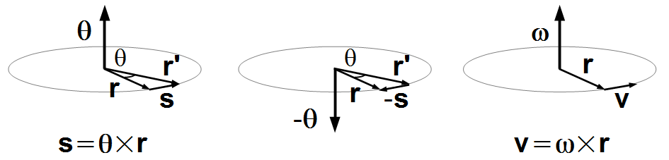 Figure 2
This is the same argument used for angular velocity, the velocity vector v is tangent to the trajectory, but the angular velocity vector ω is perpendicular to the trajectory.
This is the same argument used for angular velocity, the velocity vector v is tangent to the trajectory, but the angular velocity vector ω is perpendicular to the trajectory.
\[
\begin{gather}
\mathbf{P}={\mathbf{P}}_{T}+{\mathbf{P}}_{N}\\
\mathbf{P}=-P\operatorname{sen}\theta\;{\mathbf{e}}_{\theta}+P\cos \theta\;{\mathbf{e}}_{r}
\end{gather}
\]
The cross product
\( \mathbf{r}\times {\mathbf{F}_{g}} \)
will be
\[
\begin{gather}
\mathbf{r}\times{\mathbf{F}_{g}}=
\left|
\begin{matrix}
{\mathbf{e}}_{r} & {\mathbf{e}}_{\theta} & {\mathbf{e}}_{z}\\
a & 0 & 0\\
F_{g}\cos \theta &-F_{g}\sin \theta & 0
\end{matrix}
\right|=\\[5pt]
=[0.0-0.(-F_{g}\sin \theta)]{\mathbf{e}}_{r}-[a.0-0.F_{g}\cos\theta]{\mathbf{e}}_{\theta}+[-a F_{g}\sin \theta-0. F_{g}\cos \theta]{\mathbf{e}}_{z}\\[5pt]
\mathbf{r}\times{\mathbf{F}_{g}}=-a F_{g}\sin \theta\;{\mathbf{e}}_{z} \tag{V}
\end{gather}
\]
the gravitational force is given by
\[
\begin{gather}
\bbox[#99CCFF,10px]
{F_{g}=mg} \tag{VI}
\end{gather}
\]
substituting the value of θ and expressions (V) and (VI) into expression (IV)
\[
\begin{gather}
-amg\sin \theta\;{\mathbf{e}}_{z}=I\frac{a^{2}\theta}{dt^{2}}\;{\mathbf{e}}_{z}\\[5pt]
\frac{-{amg}}{I}\sin \theta=\frac{a^{2}\theta}{dt^{2}}
\end{gather}
\]
the equation has only components in the ez direction and setting
\( \omega ^{2}=\frac{mga}{I} \)
and writing
\( \frac{d^{2}\theta}{dt^{2}}=\ddot{\theta} \)
\[
\begin{gather}
\ddot{\theta}=-\omega ^{2}\sin \theta\\
\ddot{\theta}+\omega ^{2}\sin \theta =0
\end{gather}
\]
as we are working on a small angle approximation oscillations, we can expand the sin θ function in a
Taylor series.
Taylor series expansion of sin θ
\( \displaystyle \frac{f^{0}(0)}{0!}\theta ^{0}=\frac{\sin 0}{1}.1=0 \)
Note: \( f^{0} \) DOES NOT mean the function f to the zero power means the zero derivatives of the function f, that is, the function itself calculated in the point a.
\( \displaystyle \frac{f^{\text{I}}(0)}{1!}\theta ^{1}=\frac{\cos 0}{1}\theta =\theta \)
\( \displaystyle \frac{f^{\text{II}}(0)}{2!}\theta^{2}=\frac{-\sin 0}{2.1}\theta ^{2}=0 \)
\( \displaystyle \frac{f^{\text{III}}(0)}{3!}\theta ^{3}=\frac{-\cos 0}{3.2.1}\theta^{3}=-{\frac{\theta ^{3}}{6}} \)
\( \displaystyle \frac{f^{\text{IV}}(0)}{4!}\theta^{4}=\frac{-(-\sin 0)}{4.3.2.1}\theta ^{4}=0 \)
\( \displaystyle \frac{f^{\text{V}}(0)}{5!}\theta ^{5}=\frac{\cos 0}{5.4.3.2.1}\theta^{5}=\frac{\theta ^{5}}{120} \)
The sine function can be represented by the following series of powers
For an angle of \( 10°=\frac{\pi}{18}=0,1745 \), we have \( \sin \frac{\pi}{18}=0,1736 \), the approach represents an error of 0.5%.
\[ \bbox[#99CCFF,10px]
{f(x)=\sum _{n=0}^{\infty}{\frac{f^{n}(a)}{n!}(x-a)^{n}}}
\]
expanding around the equilibrium point with a = 0, for the first 6 terms of the series
\( \displaystyle \frac{f^{0}(0)}{0!}\theta ^{0}=\frac{\sin 0}{1}.1=0 \)
Note: \( f^{0} \) DOES NOT mean the function f to the zero power means the zero derivatives of the function f, that is, the function itself calculated in the point a.
\( \displaystyle \frac{f^{\text{I}}(0)}{1!}\theta ^{1}=\frac{\cos 0}{1}\theta =\theta \)
\( \displaystyle \frac{f^{\text{II}}(0)}{2!}\theta^{2}=\frac{-\sin 0}{2.1}\theta ^{2}=0 \)
\( \displaystyle \frac{f^{\text{III}}(0)}{3!}\theta ^{3}=\frac{-\cos 0}{3.2.1}\theta^{3}=-{\frac{\theta ^{3}}{6}} \)
\[ \displaystyle \frac{f^{\text{III}}(0)}{3!}\theta ^{3}=\frac{-\cos 0}{3.2.1}\theta^{3}=-{\frac{\theta ^{3}}{6}} \]
\( \displaystyle \frac{f^{\text{IV}}(0)}{4!}\theta^{4}=\frac{-(-\sin 0)}{4.3.2.1}\theta ^{4}=0 \)
\[ \displaystyle \frac{f^{\text{IV}}(0)}{4!}\theta^{4}=\frac{-(-\sin 0)}{4.3.2.1}\theta ^{4}=0 \]
\( \displaystyle \frac{f^{\text{V}}(0)}{5!}\theta ^{5}=\frac{\cos 0}{5.4.3.2.1}\theta^{5}=\frac{\theta ^{5}}{120} \)
\[ \displaystyle \frac{f^{\text{V}}(0)}{5!}\theta ^{5}=\frac{\cos 0}{5.4.3.2.1}\theta^{5}=\frac{\theta ^{5}}{120} \]
The sine function can be represented by the following series of powers
\[
\sin \theta =\theta -\frac{\theta ^{3}}{6}+\frac{\theta^{5}}{120}-...
\]
As we are considering θ a small angle, we can make the approach
\[
\sin \theta \approx \theta
\]
and we neglect higher-order terms.For an angle of \( 10°=\frac{\pi}{18}=0,1745 \), we have \( \sin \frac{\pi}{18}=0,1736 \), the approach represents an error of 0.5%.
\[
\ddot{\theta}+\omega ^{2}\theta =0
\]
Solution of the differential equation \( \displaystyle \ddot{\theta}+\omega^{2}\theta =0 \)
The solution is exponential type, calculating its derivatives
The solution is exponential type, calculating its derivatives
\[
\begin{array}{l}
\theta =\operatorname{e}^{\lambda t} \\
\dot{\theta}=\lambda \operatorname{e}^{\lambda t} \\
\ddot{\theta}=\lambda^{2}\operatorname{e}^{\lambda t}
\end{array}
\]
substituting in the equation
\[
\begin{gather}
\lambda ^{2}\operatorname{e}^{\lambda t}+\omega^{2}\operatorname{e}^{\lambda t}=0\\[5pt]
\lambda^{2}+\omega^{2}=0\\[5pt]
\lambda ^{2}=-\omega^{2}\\[5pt]
\lambda =\pm i\sqrt{\omega^{2}}\\[5pt]
\lambda =\pm i\omega
\end{gather}
\]
the solution is as follows, where C1 and C2 are constant
\[
\theta (t)=C_{1}\operatorname{e}^{i\omega t}+C_{2}\operatorname{e}^{-i\omega t}
\]
using Euler's formula
\( \operatorname{e}^{ix}=\cos x+i\sin x \)
\[
\begin{gather}
\theta (t)=C_{1}\left(\cos \omega t+i\sin \omega t\right)+C_{2}\left(\cos \omega t-i\sin \omega t\right)\\[5pt]
\theta(t)=\left(C_{1}+C_{2}\right)\cos \omega t-i\left(C_{2}-C_{1}\right)\sin \omega t
\end{gather}
\]
defining the following constants
\[
A=C_{1}+C_{2}\quad ,\quad B=i(C_{2}-C_{1})
\]
\[
\theta (t)=A\cos \omega t+B\sin \omega t
\]
setting
\[
\begin{array}{l}
\cos \phi=\dfrac{A}{\sqrt{A^{2}+B^{2}}}\\[5pt]
\sin \phi=\dfrac{B}{\sqrt{A^{2}+B^{2}}}\\[5pt]
\theta_{0}=\sqrt{A^{2}+B^{2}}
\end{array}
\]
substituting in the equation
\[
\begin{gather}
\theta (t)=\left(A\cos \omega t-B\sin \omega t\right)\frac{\sqrt{A^{2}+B^{2}}}{\sqrt{A^{2}+B^{2}}}\\[5pt]
\theta(t)=\sqrt{A^{2}+B^{2}}\left(\frac{A}{\sqrt{A^{2}+B^{2}}}\cos \omega t-\frac{B}{\sqrt{A^{2}+B^{2}}}\sin \omega t\right)\\[5pt]
\theta (t)=\theta_{0}\left(\cos \phi \cos \omega t-\sin \phi \sin \omega t\right)
\end{gather}
\]
The equation of motion will be
\[ \bbox[#FFCCCC,10px]
{\theta (t)=\theta _{0}\cos \left(\omega t+\phi \right)}
\]
The period of oscillations is given by
\[ \bbox[#99CCFF,10px]
{T=\frac{2\pi }{\omega}}
\]
substituting the definition of ω0 made above
\[
\begin{gather}
T=\frac{2\pi }{\sqrt{\dfrac{mga}{I}}}\\[5pt]
{T=2\pi \sqrt{\frac{I}{mga}}} \tag{VII}
\end{gather}
\]
Calculating the moment of inertia of a disk of mass m with constant density σ, the moment of
inertia relative to an axis passing through the center of mass is given by
\[
\begin{gather}
\bbox[#99CCFF,10px]
{I_{CM}=\int r^{2}\;dm} \tag{VIII}
\end{gather}
\]
Using the expression of the superficial density of mass σ, we get the mass element dm
\[
\begin{gather}
\bbox[#99CCFF,10px]
{\sigma =\frac{dm}{dA}} \tag{IX}
\end{gather}
\]
\[
\begin{gather}
dm=\sigma \;dA \tag{IX}
\end{gather}
\]
where dA is an element of angle area dθ of the disk (Figure 3)
\[
\begin{gather}
dA=r\;dr\;d\theta \tag{X}
\end{gather}
\]
substituting the expression (X) into expression (IX)
\[
\begin{gather}
dm=\sigma r\;dr\;d\theta \tag{XI}
\end{gather}
\]
substituting the expression (XI) into expression (VIII), and as integration is done on the surface of
the disk, it depends on two variables r and θ, we have a double integral
\[
I_{CM}=\iint r^{2}\sigma r\;dr\;d\theta
\]
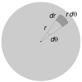
Figure 3
the density of the disk is constant, it can be moved out of the integral
\[
I_{CM}=\sigma \iint r^{3}\;dr\;d\theta
\]
The limits of integration will be from 0 to a in dr, along the radius of the disk, and from 0
to 2π in dθ, a complete turn on the disc
\[
I_{CM}=\sigma \int_{0}^{a}r^{3}\;dr\int_{0}^{2\pi}\;d\theta
\]
Integral of \( \displaystyle \int_{0}^{{a}}r^{3}dr \)
\[
\int_{0}^{{a}}r^{3}dr=\left.\frac{r^{4}}{4}\;\right|_{\;0}^{\;a}=\frac{a^{4}}{4}-\frac{0^{4}}{4}=\frac{a^{4}}{4}
\]
Integral of \( \displaystyle \int_{0}^{{2\pi}}d\theta \)
\[
\int_{0}^{{2\pi}}d\theta =\left.\theta \;\right|_{\;0}^{\;2\pi}=2\pi-0=2\pi
\]
\[
\begin{gather}
I_{CM}=\sigma \frac{a^{4}}{4}2\pi\\
I_{CM}=\sigma a^{2}\pi \frac{a^{2}}{2}
\end{gather}
\]
the factor σa2π is the total mass m of the disc (superficial density multiplied by
the disc area)
\[
\begin{gather}
I_{CM}=\frac{1}{2}ma^{2} \tag{XII}
\end{gather}
\]
This is the moment of inertia of the disk relative to the axis passing through the center of mass. The
disk on the problem, is oscillating around an axis at the edge of the disk, at a distance equal to the
radius a of the disk (Figure 4). Using the Parallel Axis Theorem
\[
\begin{gather}
\bbox[#99CCFF,10px]
{I_{p}=I_{CM}+md^{2}} \tag{XIII}
\end{gather}
\]
where d = a and substituting the expression (XII) into expression (XIII)
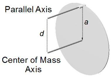
Figure 4
\[
\begin{gather}
I_{p}=\frac{1}{2}ma^{2}+ma^{2}\\
I_{p}=\frac{ma^{2}+2ma^{2}}{2}\\
I_{p}=\frac{3ma^{2}}{2} \tag{XIV}
\end{gather}
\]
substituting the expression (XIV) into expression (VII)
\[
\begin{gather}
T=2\pi\sqrt{\frac{\dfrac{3ma^{2}}{2}}{mga}}\\[5pt]
T=2\pi\sqrt{\frac{3\cancel{m}a^{\cancel{2}}}{2\cancel{m}g\cancel{a}}}
\end{gather}
\]
\[ \bbox[#FFCCCC,10px]
{T=2\pi \sqrt{\frac{3a}{2g}}}
\]
advertisement

Fisicaexe - Physics Solved Problems by Elcio Brandani Mondadori is licensed under a Creative Commons Attribution-NonCommercial-ShareAlike 4.0 International License .