Solved Problem on Waves
advertisement
Derive the Wave Equation representing a one-dimensional traveling wave on a chord of mass M and length L.
Problem data:
- String mass: M;
- String length: L.
Let us consider a long string, fixed at the ends, through which a wave propagates (Figure 1). Let us take a segment of length Δx of the chord, as the vertical displacement along the direction y is a small segment, measured in an arc over the chord, and has practically the same length as a segment measured along the x-axis. In the highlight of Figure 1, the vertical scale has been exaggerated for visualization purposes.
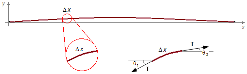
At the ends of this segment acts the tension forces T and makes angles θ1 and θ2 with the horizontal direction.
Solution
Applying Newton's Second Law
\[
\begin{gather}
\bbox[#99CCFF,10px]
{\mathbf{F}=m\mathbf{a}} \tag{I}
\end{gather}
\]
We plot the tension forces acting on the string segment on a system of coordinates (Figure 2).
Decomposing the tension forces in the z and y directions
\[
\begin{gather}
\mathbf{F}={\mathbf{T}}_{1}+{\mathbf{T}}_{2} \tag{II}
\end{gather}
\]
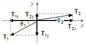
Figure 2
\[
\begin{gather}
{\mathbf{T}}_{1}=T_{1x}\;\mathbf{i}+T_{1y}\;\mathbf{j}=-T_{1}\cos\theta _{1}\;\mathbf{i}-T_{1}\sin \theta_{1}\;\mathbf{j} \tag{III}
\end{gather}
\]
\[
\begin{gather}
{\mathbf{T}}_{2}=T_{2x}\;\mathbf{i}+T_{2y}\;\mathbf{j}=T_{2}\cos\theta _{2}\;\mathbf{i}+T_{2}\sin \theta_{2}\;\mathbf{j} \tag{IV}
\end{gather}
\]
where i and j are the unit vectors in the x and y directions, substituting
expressions (III) and (IV) into expression (II)
\[
\begin{gather}
\mathbf{F}=-T_{1}\cos \theta_{1}\;\mathbf{i}-T_{1}\sin \theta_{1}\;\mathbf{j}+T_{2}\cos \theta_{2}\;\mathbf{i}+T_{2}\sin \theta_{2}\;\mathbf{j} \tag{V}
\end{gather}
\]
The acceleration of the segment will be
\[
\begin{gather}
\mathbf{a}=a_{x}\;\mathbf{i}+a_{y}\;\mathbf{j} \tag{VI}
\end{gather}
\]
substituting expressions (V) and (VI) into expression (I)
\[
\begin{gather}
-T_{1}\cos \theta_{1}\;\mathbf{i}-T_{1}\sin \theta_{1}\;\mathbf{j}+T_{2}\cos \theta_{2}\;\mathbf{i}+T_{2}\sin \theta_{2}\;\mathbf{j}=m(a_{x}\;\mathbf{i}+a_{y}\;\mathbf{j}\;)
\end{gather}
\]
Writing the components
- Direction i
\[
\begin{gather}
T_{2}\cos \theta_{2}-T_{1}\cos \theta_{1}=ma_{x}
\end{gather}
\]
in the direction x, there is no motion, the two forces balance, and the acceleration is zero,
ax = 0
\[
\begin{gather}
T_{2}\cos \theta_{2}-T_{1}\cos \theta_{1}=0\\[5pt]
T_{2}\cos\theta_{2}=T_{1}\cos \theta_{1}
\end{gather}
\]
- Direction j
\[
\begin{gather}
T_{2}\sin \theta_{2}-T_{1}\sin \theta_{1}=ma_{y}
\end{gather}
\]
letting T1 = T2 = T and writing
\( a_{y}=\frac{\partial ^{2}y}{\partial t^{2}} \),
(partial derivative was used, since the acceleration depends on two variables, x and y,
in this case, the component in x is zero.)
\[
\begin{gather}
T(\sin \theta_{2}-\sin \theta_{1})=m\frac{\partial ^{2}y}{\partial t^{2}}
\end{gather}
\]
as the vertical displacement of the string is small relative to its length, the angles
θ1 and θ2 are small (Figure 1), so we can make the
approximation
\( \sin \theta \simeq \tan \theta \) .
Note: For small angles, the value of sine and tangent are approximately equal,
e.g., for an angle
\( \theta =5°=\frac{\pi }{36}\;\text{rad} \),
we have
\( \sin \theta =0.08715574274 \)
and
\( \tan\theta =0.08748866352 \)
Note: e.g. is the abbreviation of the Latin expression "exempli gratia" which means "for example".
Note: e.g. is the abbreviation of the Latin expression "exempli gratia" which means "for example".

Figure 3
\[
\begin{gather}
T(\tan \theta_{2}-\tan\theta_{1})=m\frac{\partial ^{2}y}{\partial t^{2}} \tag{VII}
\end{gather}
\]
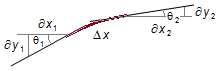
The tangent is the inclination of the straight line at the end points of the segment (Figure 4), so for
infinitesimal variations, we can write
\[
\begin{gather}
\tan \theta_{1}=\frac{\partial y_{1}}{\partial x_{1}} \tag{VIII-a}
\end{gather}
\]
\[
\begin{gather}
\tan \theta_{2}=\frac{\partial y_{2}}{\partial x_{2}} \tag{VIII-b}
\end{gather}
\]
substituting expressions (VIII-a) and (VIII-b) into expression (VII)
\[
\begin{gather}
T\left(\frac{\partial y_{2}}{\partial x_{2}}-\frac{\partial y_{1}}{\partial x_{1}}\right)=m\frac{\partial ^{2}y}{\partial t^{2}} \tag{IX}
\end{gather}
\]
The mass m of a segment Δx can be written from the expression for linear density of
mass μ
\[
\begin{gather}
\mu =\frac{m}{\Delta x}\\[5pt]
m=\mu \Delta x \tag{X}
\end{gather}
\]
substituting expression (X) into expression (IX)
\[
\begin{gather}
T\left(\frac{\partial y_{2}}{\partial x_{2}}-\frac{\partial y_{1}}{\partial x_{1}}\right)=\mu \Delta x\frac{\partial ^{2}y}{\partial t^{2}}\\[5pt]
\frac{\mu }{T}\frac{\partial^{2}y}{\partial t^{2}}=\frac{\dfrac{\partial y_{2}}{\partial x_{2}}-\dfrac{\partial y_{1}}{\partial x_{1}}}{\Delta x}
\end{gather}
\]
applying the limit to the right-hand side of the equation and letting Δx tend to zero
\[
\begin{gather}
\underset{\Delta x\rightarrow 0}{\lim }{\frac{\dfrac{\partial y_{2}}{\partial x_{2}}-\dfrac{\partial y_{1}}{\partial x_{1}}}{\Delta x}}
\end{gather}
\]
this limit represents the second derivative
\( \left(\dfrac{\partial ^{2}y}{\partial x^{2}}\right) \)
of a function y relative to x
\[
\begin{gather}
\frac{\mu}{T}\frac{\partial ^{2}y}{\partial t^{2}}=\frac{\partial^{2}y}{\partial x^{2}} \tag{XI}
\end{gather}
\]
The function y(x, t) of a wave is given by
\[
\begin{gather}
\bbox[#99CCFF,10px]
{y(x,t)=A\cos (kx-\omega t)} \tag{XII}
\end{gather}
\]
where A is the amplitude of the wave, k is the wave number, and ω is the angular
frequency, to determine the ratio
\( \frac{\mu}{T} \)
we derive expression (XII) twice, relative to position x relative to time t.
Partial derivative relative to x of \( y(x,t)=A\cos (kx-\omega t) \)
in this case, the time t is constant, and the function y(x, t) is a composite function, using the Chain Rule
in this case, the time t is constant, and the function y(x, t) is a composite function, using the Chain Rule
\[
\begin{gather}
\frac{\partial y[v(x)]}{\partial x}=\frac{dy}{dv}\frac{dv}{dx}
\end{gather}
\]
with
\( y(v)=A\cos v \)
and
\( v(x)=kx-\omega t \)
\[
\begin{array}{l}
\dfrac{dy}{dv}=-A\sin v=-A\sin (kx-\omega t) \\[5pt]
\dfrac{dv}{dx}=k
\end{array}
\]
\[
\begin{gather}
\frac{\partial y}{\partial x}=-Ak\sin (kx-\omega t)
\end{gather}
\]
differentiating a second time with respect to x, again using the chain rule
\[
\begin{gather}
\frac{\partial ^{2}y[v(x)]}{\partial x^{2}}=\frac{dy}{dv}\frac{dv}{dx}
\end{gather}
\]
with
\( y(v)=-Ak\sin v \)
and
\( v(x)=kx-\omega t \),
the derivatives will be
\[
\begin{array}{l}
\dfrac{dy}{dv}=-Ak\cos v=-Ak\cos (kx-\omega t) \\[5pt]
\dfrac{dv}{dx}=k
\end{array}
\]
\[
\begin{gather}
\frac{\partial ^{2}y}{\partial x^{2}}=-A k^{2}\cos (kx-\omega t)
\end{gather}
\]
Partial derivative relative to t of \( y(x,t)=A \cos (kx-\omega t) \)
in this case the displacement x is constant and the function y(x, t) is a composite function, using the Chain Rule
in this case the displacement x is constant and the function y(x, t) is a composite function, using the Chain Rule
\[
\begin{gather}
\frac{\partial y[v(t)]}{\partial t}=\frac{dy}{dv}\frac{dv}{dt}
\end{gather}
\]
with
\( y(v)=A\cos v \)
and t
\( v(t)=kx-\omega t \),
the derivatives will be
\[
\begin{array}{l}
\dfrac{dy}{dv}=-A\sin v=-A\sin (kx-\omega t)\\[5pt]
\dfrac{dv}{dt}=\omega
\end{array}
\]
\[
\begin{gather}
\frac{\partial y}{\partial t}=-A\omega \sin (kx-\omega t)
\end{gather}
\]
differentiating a second time relative to t, again using the chain rule
\[
\begin{gather}
\frac{\partial ^{2}y[v(t)]}{\partial t^{2}}=\frac{dy}{dv}\frac{dv}{dt}
\end{gather}
\]
with
\( y(v)=-A\omega \sin v \)
and
\( v(t)=kx-\omega t \),
the derivatives will be
\[
\begin{array}{l}
\dfrac{dy}{dv}=-A\omega \cos v=-A\omega \cos (kx-\omega t)\\[5pt]
\dfrac{dv}{dt}=\omega
\end{array}
\]
\[
\begin{gather}
\frac{\partial ^{2}y}{\partial t^{2}}=-A\omega ^{2}\cos (kx-\omega t)
\end{gather}
\]
Substituting these derivatives into expression (XI)
\[
\begin{gather}
-{\frac{\mu}{T}}\cancel{A}\omega ^{2}\cancel{\cos (kx-\omega t)}=\cancel{A}k^{2}\cancel{\cos (kx-\omega t)}\\[5pt]
\frac{\mu }{T}\omega^{2}=k^{2}\\[5pt]
\frac{\mu }{T}=\frac{k^{2}}{\omega^{2}}=\left(\frac{k}{\omega}\right)^{2}
\end{gather}
\]
The speed of a wave as a function of wave number and angular frequency is given by
\[
\begin{gather}
v=\frac{\omega }{k}\\[5pt]
\frac{1}{v}=\frac{k}{\omega}\\[5pt]
\left(\frac{k}{\omega}\right)^{2}=\frac{1}{v^{2}} \tag{XIII}
\end{gather}
\]
substituting expression (XIII) into expression (XI)
\[
\begin{gather}
\bbox[#FFCCCC,10px]
{\frac{\partial ^{2}y}{\partial x^{2}}=\frac{1}{v^{2}}\frac{\partial^{2}y}{\partial t^{2}}}
\end{gather}
\]
advertisement

Fisicaexe - Physics Solved Problems by Elcio Brandani Mondadori is licensed under a Creative Commons Attribution-NonCommercial-ShareAlike 4.0 International License .