Solved Problem on Harmonic Oscillations
advertisement
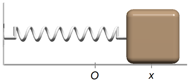
A block of mass m is attached to the end of a spring, the spring constant is equal to k,
and placed on a horizontal frictionless surface. The other end of the spring is fixed at a point in the
wall. The block is displaced from its equilibrium position and released. Determine:
a) The equation of motion of the block;
b) The velocity as a function of the mass, m, the spring constant, k, the amplitude, A, and the distance, x, between the block and the point of equilibrium of the spring;
c) The magnitude of the maximum speed;
d) The acceleration as a function of the mass, m, the spring constant, k, and the distance, x, between the block and the point of equilibrium of the spring;
e) The magnitude of the maximum acceleration;
f) The kinetic energy;
g) The potential energy;
h) The total energy.
Problem data:
- Block mass: m;
- Spring constant: k.
We choose a reference frame with a positive direction to the right. The block is displaced and released,
and the spring force will act to restore the equilibrium position (Figure 1).
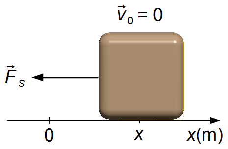
a) Applying Newton's Second Law (Figure 1)
\[
\begin{gather}
\bbox[#99CCFF,10px]
{F=m\frac{d^{2}x}{dt^{2}}} \tag{I}
\end{gather}
\]
the force acting on the block is the spring force
\( {\vec{F}}_{S} \)
given, in magnitude, by
\[
\begin{gather}
\bbox[#99CCFF,10px]
{F_{S}=-kx} \tag{II}
\end{gather}
\]
the minus sign in the spring force indicates that it acts in the opposite direction of displacement
of the block (acts in the direction of restoring equilibrium). Substituting the expression (II) into
expression (I)
\[
\begin{gather}
-kx=m\frac{d^{2}x}{dt^{2}}\\[5pt]
m\frac{d^{2}x}{dt^{2}}+kx=0
\end{gather}
\]
that is a Second Order Homogeneous Ordinary Differential Equation. Dividing the equation by the
mass m
\[
\begin{gather}
\frac{d^{2}x}{dt^{2}}+\frac{k}{m}x=0
\end{gather}
\]
setting the definition
\( \omega_{0}^{2}\equiv \frac{k}{m} \)
\[
\begin{gather}
\frac{d^{2}x}{dt^{2}}+\omega_{0}^{2}x=0
\end{gather}
\]
Solution of \( \displaystyle \frac{d^{2}x}{dt^{2}}+\omega_{0}^{2}x=0 \)
The solution to this type of equation is found substituting
The solution to the differential equation will be
The solution to this type of equation is found substituting
\[
\begin{array}{l}
x=\operatorname{e}^{\lambda t}\\[5pt]
\dfrac{dx}{dt}=\lambda\operatorname{e}^{\lambda t}\\[5pt]
\dfrac{d^{2}x}{dt^{2}}=\lambda^{2}\operatorname{e}^{\lambda t}
\end{array}
\]
substituting these values into the differential equation
\[
\begin{gather}
\lambda^{2}\operatorname{e}^{\lambda t}+\omega_{0}^{2}\operatorname{e}^{\lambda t}=0\\[5pt]
\operatorname{e}^{\lambda t}\left(\lambda^{2}+\omega_{0}^{2}\right)=0\\[5pt]
\lambda^{2}+\omega_{0}^{2}=\frac{0}{\operatorname{e}^{\lambda t}}\\[5pt]
\lambda^{2}+\omega_{0}^{2}=0
\end{gather}
\]
this is the Characteristic Equation that has a solution
\[
\begin{gather}
\lambda ^{2}=-\omega_{0}^{2}\\[5pt]
\lambda =\sqrt{-\omega_{0}^{2}}\\[5pt]
\lambda _{1,2}=\pm \omega_{0}\mathsf{i}
\end{gather}
\]
where \( \mathsf{i}=\sqrt{-1\;} \).The solution to the differential equation will be
\[
\begin{gather}
x=C_{1}\operatorname{e}^{\lambda_{1}t}+C_{2}\operatorname{e}^{\lambda_{2}t}\\[5pt]
x=C_{1}\operatorname{e}^{\omega_{0}\mathsf{i}t}+C_{2}\operatorname{e}^{-\omega_{0}\mathsf{i}t}
\end{gather}
\]
where C1 and C2 are constants of integration, using
Euler's Formula
\( \operatorname{e}^{i\theta }=\cos \theta+\mathsf{i}\sin \theta \)
\[
\begin{gather}
x=C_{1}\left(\cos \omega_{0}t+\mathsf{i}\sin \omega_{0}t\right)+C_{2}\left(\cos\omega_{0}t-\mathsf{i}\sin \omega_{0}t\right)\\[5pt]
x=C_{1}\cos \omega_{0}t+\mathsf{i}C_{1}\sin \omega_{0}t+C_{2}\cos \omega_{0}t-\mathsf{i}C_{2}\sin \omega_{0}t\\[5pt]
x=\left(C_{1}+C_{2}\right)\cos \omega_{0}t+\mathsf{i}\left(C_{1}-C_{2}\right)\sin \omega_{0}t
\end{gather}
\]
defining two new constants α and β in terms of C1 e
C2
\[
\begin{gather}
\alpha \equiv C_{1}+C_{2}\\[5pt]
\text{e}\\[5pt]
\beta \equiv \mathsf{i}(C_{1}-C_{2})
\end{gather}
\]
\[
\begin{gather}
x=\alpha \cos \omega_{0}t+\beta \sin \omega_{0}t
\end{gather}
\]
multiplying and dividing this expression by
\( \sqrt{\alpha ^{2}+\beta ^{2}} \)
\[
\begin{gather}
x=\left(\alpha \cos \omega_{0}t+\beta\sin \omega_{0}t\right)\frac{\sqrt{\alpha ^{2}+\beta^{2}\;}}{\sqrt{\alpha ^{2}+\beta ^{2}\;}}\\[5pt]
x=\sqrt{\alpha ^{2}+\beta^{2}\;}\left(\frac{\alpha }{\sqrt{\alpha ^{2}+\beta ^{2}}}\cos \omega_{0}t+\frac{\beta }{\sqrt{\alpha ^{2}+\beta^{2}\;}}\sin \omega_{0}t\right)
\end{gather}
\]
setting
\[
\begin{align}
& A\equiv \sqrt{\alpha^{2}+\beta^{2}\;}\\[5pt]
& \cos \varphi \equiv \frac{\alpha}{\sqrt{\alpha^{2}+\beta^{2}\;}}\\[5pt]
& \sin \varphi \equiv \frac{\beta }{\sqrt{\alpha^{2}+\beta^{2}\;}}
\end{align}
\]
\[
\begin{gather}
x=A(\cos \varphi \cos \omega_{0}t+\sin \varphi\sin \omega_{0}t)
\end{gather}
\]
From the trigonometric identity
\( \cos(a-b)=\cos a\cos b+\sin a\sin b .\)
\[ \cos(a-b)=\cos a\cos b+\sin a\sin b \]
\[
\begin{gather}
\bbox[#FFCCCC,10px]
{x=A\cos (\omega_{0}t-\varphi )}
\end{gather}
\]
b) The speed is given by
\[
\begin{gather}
\bbox[#99CCFF,10px]
{v=\frac{dx}{dt}}
\end{gather}
\]
Differentiation of \( x=A\cos (\omega_{0}t-\varphi ) \)
the function x(t)) is a composite function using the Chain Rule
the function x(t)) is a composite function using the Chain Rule
\[
\begin{gather}
\frac{dx[u(t)]}{dt}=\frac{dx}{du}\frac{du}{dt}
\end{gather}
\]
with
\( x(u)=A\cos u \)
and
\( u(t)=\omega_{0}t-\varphi \)
\[
\begin{gather}
\frac{dx}{dt}=\frac{dx}{du}\frac{du}{dt}\\[5pt]
\frac{dx}{dt}=\frac{d(A \cos u)}{du}\frac{d(\omega_{0}t-\varphi)}{dt}\\[5pt]
\frac{dx}{dt}=A (-\sin u)(\omega_{0})\\[5pt]
\frac{dx}{dt}=-\omega_{0}A\sin (\omega_{0}t-\varphi)
\end{gather}
\]
\[
\begin{gather}
v=-\omega_{0}A\sin (\omega_{0}t-\varphi ) \tag{III}
\end{gather}
\]
From the trigonometric identity
\( \cos ^{2}\theta +\sin ^{2}\theta=1 \)
\[
\begin{gather}
\sin \theta =\sqrt{1-\cos ^{2}\theta \;}
\end{gather}
\]
\[
\begin{gather}
v=-\omega_{0}A\sqrt{1-\cos ^{2}(\omega_{0}t-\varphi)}\\[5pt]
v=-\sqrt{\omega_{0}^{2}A^{2}[1-\cos ^{2}(\omega_{0}t-\varphi)]} \tag{IV}
\end{gather}
\]
writing the solution to part (a) in the form as follow and squaring both sides of the equation
\[
\begin{gather}
\cos (\omega_{0}t-\varphi )=\frac{x}{A}\\[5pt]
\cos^{2}(\omega_{0}t-\varphi )=\frac{x^{2}}{A^{2}} \tag{V}
\end{gather}
\]
substituting the expression (V) into (IV) and the definition of
\( \omega_{0}^{2} \)
made above
\[
\begin{gather}
v=-\sqrt{\frac{k}{m}A^{2}\left(1-\frac{x^{2}}{A^{2}}\right)}\\[5pt]
v=-\sqrt{\frac{k}{m}A^{2}\left(\frac{A^{2}-x^{2}}{A^{2}}\right)}
\end{gather}
\]
\[
\begin{gather}
\bbox[#FFCCCC,10px]
{v=-\sqrt{\frac{k}{m}\left(A^{2}-x^{2}\right)}}
\end{gather}
\]
c) In the solution of item (b) analyzing the term in parentheses \( \left(A^{2}-x^{2}\right) \), we have that x2 is always positive, therefore this term will have a maximum value for x = 0, so the magnitude of the maximum speed will be
\[
\begin{gather}
\left|\;v_{max}\;\right|=\sqrt{\frac{k}{m}\left(A^{2}-0^{2}\right)}\\[5pt]
\left|\;v_{max}\;\right|=\sqrt{\frac{k}{m}A^{2}}
\end{gather}
\]
\[
\begin{gather}
\bbox[#FFCCCC,10px]
{\left|\;v_{max}\;\right|=A\sqrt{\frac{k}{m}\;}}
\end{gather}
\]
d) The acceleration is given by
\[
\begin{gather}
\bbox[#99CCFF,10px]
{a=\frac{dv}{dt}}
\end{gather}
\]
differentiating the expression (III) from item (b)
Differentiation of \( v=-\omega_{0}A\sin (\omega_{0}t-\varphi ) \)
the function v(t)) is a composite function using the Chain Rule
the function v(t)) is a composite function using the Chain Rule
\[
\begin{gather}
\frac{dv[u(t)]}{dt}=\frac{dv}{du}\frac{du}{dt}
\end{gather}
\]
with
\( v(u)=-\omega_{0}A\sin u \)
and
\( u(t)=\omega_{0}t-\varphi \)
\[
\begin{gather}
\frac{dv}{dt}=\frac{dv}{du}\frac{du}{dt}\\[5pt]
\frac{dv}{dt}=\frac{d(-\omega_{0}A\sin u)}{du}\frac{d(\omega_{0}t-\varphi)}{dt}\\[5pt]
\frac{dv}{dt}=\omega_{0}A (-\sin u)(\omega_{0})\\[5pt]
\frac{dv}{dt}=-\omega_{0}^{2}A\cos (\omega_{0}t-\varphi)
\end{gather}
\]
\[
\begin{gather}
a=-\omega_{0}^{2}A\cos (\omega_{0}t-\varphi )
\end{gather}
\]
comparing this expression with the solution of the part (a) and with the definition of
\( \omega_{0}^{2} \)
made above
\[
a=-\frac{{k}}{m}\underbrace{A\cos (\omega_{0}t-\varphi )}_{x}
\]
\[
\begin{gather}
\bbox[#FFCCCC,10px]
{a=-\frac{{k}}{m}x}
\end{gather}
\]
e) The maximum acceleration occurs for the maximum value of x, which occurs when the amplitude is maximum, x = A
\[
\begin{gather}
\bbox[#FFCCCC,10px]
{\left|\;a_{max}\;\right|=-{\frac{k}{m}}A}
\end{gather}
\]
f) The kinetic energy is given by
\[
\begin{gather}
\bbox[#99CCFF,10px]
{K=\frac{mv^{2}}{2}} \tag{VI}
\end{gather}
\]
substituting expression (III) into expression (VI)
\[
\begin{gather}
K=\frac{m\left(-\omega_{0}A\sin (\omega_{0}t-\varphi)\right)^{2}}{2}\\[5pt]
K=\frac{m\omega_{0}^{2}A^{2}\sin ^{2}(\omega_{0}t-\varphi)}{2}
\end{gather}
\]
substituting the definition of
\( \omega_{0}^{2} \)
made above
\[
\begin{gather}
K=\frac{m\left(-\omega_{0}A\sin (\omega_{0}t-\varphi)\right)^{2}}{2}\\[5pt]
K=m \omega_{0}^{2} \frac{A^{2}\sin ^{2}(\omega_{0}t-\varphi )}{2}\\[5pt]
K=\cancel{m}\frac{k}{\cancel{m}}\frac{A^{2}\sin ^{2}(\omega_{0}t-\varphi )}{2}
\end{gather}
\]
\[
\begin{gather}
\bbox[#FFCCCC,10px]
{K=\frac{kA^{2}}{2}\sin ^{2}(\omega_{0}t-\varphi )}
\end{gather}
\]
g) The elastic potential energy is given by
\[
\begin{gather}
\bbox[#99CCFF,10px]
{U=\frac{kx^{2}}{2}} \tag{VII}
\end{gather}
\]
substituting the solution of the item (a) into expression (VII)
\[
\begin{gather}
U=\frac{k\left[A\cos (\omega_{0}t-\varphi )\right]^{2}}{2}
\end{gather}
\]
\[
\begin{gather}
\bbox[#FFCCCC,10px]
{U=\frac{kA^{2}}{2}\cos ^{2}(\omega_{0}t-\varphi )}
\end{gather}
\]
h) The total energy will be given by the sum of the results of items (f) and (g)
\[
\begin{gather}
\bbox[#99CCFF,10px]
{E=K+U}
\end{gather}
\]
\[
\begin{gather}
E=\frac{kA^{2}}{2}\sin ^{2}(\omega_{0}t-\varphi )+\frac{kA^{2}}{2}\cos ^{2}(\omega_{0}t-\varphi)\\[5pt]
E=\frac{kA^{2}}{2}\left[\underbrace{\sin ^{2}(\omega_{0}t-\varphi )+\cos ^{2}(\omega_{0}t-\varphi )}_{1}\right]
\end{gather}
\]
\[
\begin{gather}
\bbox[#FFCCCC,10px]
{E=\frac{kA^{2}}{2}}
\end{gather}
\]
advertisement

Fisicaexe - Physics Solved Problems by Elcio Brandani Mondadori is licensed under a Creative Commons Attribution-NonCommercial-ShareAlike 4.0 International License .