Solved Problem on Harmonic Oscillations
advertisement
A block of mass m = 0.25 kg is connected to a spring of constant k = 0.25 N/m
and a shock absorber of damping coefficient b = 0.5 N.S/m. The block is displaced from its
equilibrium position to a point P to 0.1 m and released from rest. Determine:
a) Equation of displacement as a function of time;
b) What is the type of oscillation;
c) The graph of positon x as a function of time t.
a) Equation of displacement as a function of time;
b) What is the type of oscillation;
c) The graph of positon x as a function of time t.

Problem data:
- Mass of the body: m = 0.25 kg;
- Spring constant: k = 0.25 N/m;
- Damping coefficient: b = 0.5 N.s/m;
- Initial position (t = 0): x0 = 0.1 m;
- Initial velocity (t = 0): v0 = 0.
We choose a frame of reference with a positive direction to the right. The block is displaced to
position x0 = 0.1 m, and when released, the spring force will return the block to the
equilibrium position. The initial velocity is equal to zero, v0 = 0. Writing the
Initial Conditions of the problem
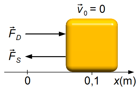
Figure 1
\[
\begin{array}{l}
x(0)=0.1\;\text{m}\\[10pt]
v_{0}=\dfrac{dx(0)}{dt}=0
\end{array}
\]
Solution
a) Applying Newton's Second Law
\[
\begin{gather}
\bbox[#99CCFF,10px]
{F=m\frac{d^{2}x}{dt^{2}}} \tag{I}
\end{gather}
\]
the spring force is given by
\[
\begin{gather}
\bbox[#99CCFF,10px]
{F_{S}=-kx} \tag{II-a}
\end{gather}
\]
the damping force is given by
\[
\begin{gather}
\bbox[#99CCFF,10px]
{F_{D}=-bv=-b\frac{dx}{dt}} \tag{II-b}
\end{gather}
\]
The negative sign in spring force represents that it acts in the opposite direction of block
displacement (acts to restore the equilibrium), and in the damping force represents that it acts
against the direction of speed (acts to brake the movement). Substituting the expressions (II-a)
and (II-b) into expression (I)
\[
\begin{gather}
-F_{S}-F_{D}=m\frac{d^{2}x}{dt^{2}}\\[5pt]
-kx-b\frac{dx}{dt}=m\frac{d^{2}x}{dt^{2}}\\[5pt]
m\frac{d^{2}x}{dt^{2}}+b\frac{dx}{dt}+kx=0
\end{gather}
\]
that is a Second-Order Linear Homogeneous Differential Equation. Dividing the equation by the
mass m
\[
\begin{gather}
\frac{d^{2}x}{dt^{2}}+\frac{b}{m}\frac{dx}{dt}+\frac{k}{m}x=0
\end{gather}
\]
substituting the values given in the problem
\[
\begin{gather}
\frac{d^{2}x}{dt^{2}}+\frac{0.5}{0.25}\frac{dx}{dt}+\frac{0.25}{0.25}x=0\\[5pt]
\frac{d^{2}x}{dt^{2}}+2\frac{dx}{dt}+x=0 \tag{III}
\end{gather}
\]
Solution of \( \displaystyle \frac{d^{2}x}{dt^{2}}+2\frac{dx}{dt}+x=0 \)
The solution to this type of equation is found by substituting
Differentiating the expression (IV) with respect to time, the function x(t) is a sum of two functions, and the derivative of a sum is the sum of derivatives
The solution to this type of equation is found by substituting
\[
\begin{array}{l}
x={\operatorname{e}}^{\lambda t}\\[5pt]
\dfrac{dx}{dt}=\lambda {\operatorname{e}}^{\lambda t}\\[5pt]
\dfrac{d^{2}x}{dt^{2}}=\lambda^{2}{\operatorname{e}}^{\lambda t}
\end{array}
\]
substituting this values into the differential equation
\[
\begin{gather}
\lambda^{2}{\operatorname{e}}^{\lambda t}+2\lambda{\operatorname{e}}^{\lambda t}+{\operatorname{e}}^{\lambda t}=0\\[5pt]
{\operatorname{e}}^{\lambda t}\left(\lambda^{2}+2\lambda+1\right)=0\\[5pt]
\lambda^{2}+2\lambda+1=\frac{0}{{\operatorname{e}}^{\lambda t}}\\[5pt]
\lambda^{2}+2\lambda+1=0
\end{gather}
\]
that is the Characteristic Equation that has as its solution
\[
\begin{gather}
\Delta =b^{2}-4ac=2^{2}-4\times 1\times 1=4-4=0\\[10pt]
\lambda_{1}=\lambda_{2}=\frac{-b}{2a}=\frac{-2}{2\times 1}=\frac{-2}{2}=-1
\end{gather}
\]
as Δ = 0, the solution of the differential equation will be
\[
\begin{gather}
x=C_{1}{\operatorname{e}}^{\lambda_{1}t}+C_{2}t{\operatorname{e}}^{\lambda_{2}t}\\[5pt]
x=C_{1}{\operatorname{e}}^{-t}+C_{2}t{\operatorname{e}}^{-t} \tag{IV}
\end{gather}
\]
where C1 and C2 are constant of integration determined by the
Initial Conditions.Differentiating the expression (IV) with respect to time, the function x(t) is a sum of two functions, and the derivative of a sum is the sum of derivatives
\[
\begin{gather}
(f+g)'=f'+g'
\end{gather}
\]
the second term on the right-hand side of the equation is the product of two functions, using the
product rule for derivatives
\[
\begin{gather}
(uv)'=u'v+uv'
\end{gather}
\]
with
\( f=C_{1}{\operatorname{e}}^{-t} \),
\( g=C_{2}t{\operatorname{e}}^{-t} \)
and
\( u=t \),
\( v={\operatorname{e}}^{-t} \),
\[
\begin{gather}
\frac{dx}{dt}=\frac{df}{dt}+\frac{dg}{dt}\\[5pt]
\frac{dx}{dt}=\frac{df}{dt}+\left(\frac{du}{dt}v+u\frac{dv}{dt}\right)\\[5pt]
\frac{dx}{dt}=\left(-C_{1}{\operatorname{e}}^{-t}\right)+\left[1.{C_{2}\operatorname{e}}^{-t}+\left({-tC_{2}\operatorname{e}}^{-t}\right)\right]\\[5pt]
\frac{dx}{dt}=-C_{1}{\operatorname{e}}^{-t}+C_{2}{\operatorname{e}}^{-t}-C_{2}t{\operatorname{e}}^{-t}\\[5pt]
\frac{dx}{dt}=-C_{1}{\operatorname{e}}^{-t}+C_{2}{\operatorname{e}}^{-t}\left(1-t\right) \tag{V}
\end{gather}
\]
substituting the Initial Conditions into expressions (IV) and (V)
\[
\begin{gather}
x(0)=0.1=C_{1}{\operatorname{e}}^{-0}+C_{2}.0.{\operatorname{e}}^{-0}\\[5pt]
0.1=C_{1}{\operatorname{e}}^{0}+0\\[5pt]
C_{1}=0,1 \tag{VI}
\end{gather}
\]
\[
\begin{gather}
\frac{dx(0)}{dt}=0=-C_{1}{\operatorname{e}}^{-0}+C_{2}{\operatorname{e}}^{-0}\left(1-0\right)\\[5pt]
0=-C_{1}{\operatorname{e}}^{0}+C_{2}{\operatorname{e}}^{0}1\\[5pt]
0=-C_{1}+C_{2}
\end{gather}
\]
substituting the value of C1 found in (VI)
\[
\begin{gather}
0=-0.1+C_{2}\\[5pt]
C_{2}=0.1 \tag{VII}
\end{gather}
\]
substituting these constants in the expression (IV)
\[
\begin{gather}
x(t)=0.1{\operatorname{e}}^{-t}+0.1t{\operatorname{e}}^{-t}
\end{gather}
\]
\[
\begin{gather}
\bbox[#FFCCCC,10px]
{x(t)=0.1{\operatorname{e}}^{-t}\left(1+t\right)}
\end{gather}
\]
b) As Δ = 0, the oscillator is critically damped.
c) Plotting the graph of
\[
\begin{gather}
x(t)=0.1{\operatorname{e}}^{-t}\left(1+t\right) \tag{VIII}
\end{gather}
\]
Setting x(t) = 0 in the expression (VIII), we find the roots of the equation
Differentiating \( x(t)=0,1{\operatorname{e}}^{-t}\left(1+t\right) \)
The function x(t) is given by the product of two functonss, using again, the rule of product for derivatives, with \( u=0,1\operatorname{e}^{-t} \) and \( v=1+t \)
Differentiating a second time the function.
Differentiation of \( \dfrac{dx}{dt}=-0,1t{\operatorname{e}}^{-t} \), using again, the rule of product for derivatives, with \( u=-0,1t \) e \( v={\operatorname{e}}^{-t} \)
Since the variable t represents the time, we do not calculate negative values (t < 0), to tend to infinity
\[
\begin{gather}
x(t)=0.1{\operatorname{e}}^{-t}\left(1+t\right)=0\\[5pt]
0.1{\operatorname{e}}^{-t}\left(1+t\right)=0
\end{gather}
\]
we have the roots when
\( 0.1{\operatorname{e}}^{-t}=0 \)
or
\( 1+t=0 \),
in the first case, there is no t that satisfies the equation, in the second case, the
function x(t) intercepts the abscissa axis at t = −1, and there is a root
in the point (t, x) = (-1, 0).
Differentiating \( x(t)=0,1{\operatorname{e}}^{-t}\left(1+t\right) \)
The function x(t) is given by the product of two functonss, using again, the rule of product for derivatives, with \( u=0,1\operatorname{e}^{-t} \) and \( v=1+t \)
\[
\begin{gather}
\frac{dx}{dt}=\frac{du}{dt}v+u\frac{dv}{dt}\\[5pt]
\frac{dx}{dt}=-0,1{\operatorname{e}}^{-t}(1+t)+0,1{\operatorname{e}}^{-t}.1=\\[5pt]
\frac{dx}{dt}=-0,1{\operatorname{e}}^{-t}-0,1{\operatorname{e}}^{-t}t+0,1{\operatorname{e}}^{-t}=\\[5pt]
\frac{dx}{dt}=-0,1{\operatorname{e}}^{-t}t \tag{IX}
\end{gather}
\]
setting
\( \dfrac{dx(t)}{dt}=0 \),
we find the maximum and minimum points of the function
\[
\begin{gather}
-0.1t{\operatorname{e}}^{-t}=0
\end{gather}
\]
we have the roots when
\( 0.1{\operatorname{e}}^{-t}=0 \)
or t = 0, in the first case, there is no t that satisfies equality, in the second
case, substituting t = 0 into the expression (VIII)
\[
\begin{gather}
x(0)=0.1{\operatorname{e}}^{-0}\left(1+0\right)\\[5pt]
x=0.1
\end{gather}
\]
there is a maximum or minimum point in (t, x) = (0, 0.1). For negative t values
(t < 0), the derivative will always be positive
\( \left(\dfrac{dx(t)}{dt}>0\right) \),
and the function grows. For positive t values (t > 0), the derivative will always be
negative
\( \left(\dfrac{dx(t)}{dt}<0\right) \),
and the function decreases.Differentiating a second time the function.
Differentiation of \( \dfrac{dx}{dt}=-0,1t{\operatorname{e}}^{-t} \), using again, the rule of product for derivatives, with \( u=-0,1t \) e \( v={\operatorname{e}}^{-t} \)
\[
\begin{gather}
\frac{d^{2}x}{dt^{2}}=\frac{du}{dt}v+u\frac{dv}{dt}\\[5pt]
\frac{d^{2}x}{dt^{2}}=-0,1{\operatorname{e}}^{-t}+(-0,1t)(-{\operatorname{e}}^{-t})=\\[5pt]
\frac{d^{2}x}{dt^{2}}=-0,1{\operatorname{e}}^{-t}+0,1t{\operatorname{e}}^{-t}=\\[5pt]
\frac{d^{2}x}{dt^{2}}=0,1{\operatorname{e}}^{-t}(-1+t) \tag{X}
\end{gather}
\]
setting
\( \dfrac{d^{2}x(t)}{dt^{2}}=0 \),
we find inflection points in the function
\[
\begin{gather}
0.1{\operatorname{e}}^{-t}\left(-1+t\right)=0
\end{gather}
\]
we have the roots when
\( 0.1{\operatorname{e}}^{-t}=0 \)
or
\( -1+t=0 \),
in the first case, there is no t that satisfies the equality, in the second case, we have
t = 1, substituting this value into the expression (VIII)
\[
\begin{gather}
x(1)=0.1{\operatorname{e}}^{-1}\left(1+1\right)\\[5pt]
x(1)=0.1\times 0.37\times 2\\[5pt]
x=0.074
\end{gather}
\]
there is an inflection point in (t, x) = (1, 0.074). For values of t less than 1
(t < 1), the second derivative will always be negative
\( \left(\dfrac{d^{2}x(t)}{dt^{2}}<0\right) \),
and the function has a concave downward, for values of t greater than 1 (t > 1), the
second derivative will always be positive
\( \left(\dfrac{d^{2}x(t)}{dt^{2}}>0\right) \),
and the function has a concave upwards. As the graph has a concave downward to t less than 1, the
point (t, x) = (0, 0.1) found in the first derivative is the maximum point.Since the variable t represents the time, we do not calculate negative values (t < 0), to tend to infinity
\[
\begin{gather}
\lim _{t\rightarrow \infty }x(t)=\lim _{t\rightarrow \infty}0.1{\operatorname{e}}^{-t}\left(1+t\right)=\lim _{t\rightarrow \infty}{\frac{0.1}{{\operatorname{e}}^{-t}}}\left(1+t\right)=\frac{0.1}{{\operatorname{e}}^{-\infty}}\left(1+\infty \right)=0
\end{gather}
\]
The function
\( \dfrac{0.1}{{\operatorname{e}}^{-\infty }} \)
tends to zero, and the expression
\( \left(1+\infty \right) \)
tends to infinity, as the exponential converges faster, the function limit tends to zero.
From the analysis done above, we plot the graph of the displacement as a function of time (Graph 1).

advertisement

Fisicaexe - Physics Solved Problems by Elcio Brandani Mondadori is licensed under a Creative Commons Attribution-NonCommercial-ShareAlike 4.0 International License .