Solved Problem on Gauss's Law

Determine the magnitude of the electric field produced by a thin spherical shell, of radius R and electric charge Q>0, everywhere in the space.

Problem data:

Radius of spherical shell: R.
Charge of the spherical shell: Q.

Problem diagram:

To determine the magnitude of the electric field everywhere in space, we must consider the points inside the spherical shell, r ≤ R, and points outside the spherical shell, r > R, (Figure 1).

Figure 1

We construct an internal Gaussian Surface and another surface external to the spherical shell.

Solution

For r ≤ R:

Inside the spherical shell, there are no charges, the electric field is zero

\[ \bbox[#FFCCCC,10px] {E=0} \]

For r > R:

Gauss's Law is given by

\[ \begin{gather} \bbox[#99CCFF,10px] {\oint_{A}{\mathbf{E}}.d\mathbf{A}=\frac{q}{\epsilon_{0}}} \tag{I} \end{gather} \]

The electric field spreads radially from the charge distribution in the e_r direction, and in each surface area element dA, we have a unit vector n perpendicular to the surface and oriented outwards. Thus, at each point on the surface, the electric field vector E and the unit vector n have the same direction (Figure 2).

Figure 2

The electric field vector only has a component in the e_r direction, it can be written as

\[ \begin{gather} \mathbf{E}=E{\;\mathbf{e}}_{r} \tag{II} \end{gather} \]

The area element vector can be written as

\[ \begin{gather} d\mathbf{A}=dA\;\mathbf{n} \tag{III} \end{gather} \]

substituting expressions (II) and (III) into expression (I)

\[ \begin{gather} \oint_{A}E\;{\mathbf{e}}_{r}.dA\;\mathbf{n}=\frac{q}{\epsilon_{0}}\\ \oint_{A}E\;dA\;\underbrace{{\mathbf{e}}_{r}.\mathbf{n}}_{1}=\frac{q}{\epsilon_{0}} \end{gather} \]

Note: As e_r and n are unit vectors, their magnitudes are equal to 1, and as both are in the same direction, the angle between them is zero, θ=0, \( {\mathbf{e}}_{r}.\mathbf{n}=|\;\mathbf{e}_{r}\;|\;|\;\mathbf{n}\;|\;\cos 0=1.1.1=1 \)

\[ {\mathbf{e}}_{r}.\mathbf{n}=|\;\mathbf{e}_{r}\;|\;|\;\mathbf{n}\;|\;\cos 0=1.1.1=1 \]

\[ \begin{gather} \oint _{A}E\;dA=\frac{q}{\epsilon_{0}} \tag{IV} \end{gather} \]

The area element dA will be (Figure 3-A)

\[ \begin{gather} dA=r\;d\theta \;r\sin \theta \;d\phi\\ dA=r^{2}\;\sin \theta \;d\theta \;d\phi \tag{V} \end{gather} \]

substituting expression (V) into expression (VI)

\[ \begin{gather} \int_{A}Er^{2}\sin \theta \;d\theta \;d\phi =\frac{q}{\epsilon_{0}} \tag{VI} \end{gather} \]

Since the electric field is uniform and the integral does not depend on the radius, they can be moved out of the integral and the integrals can be separated.

\[ Er^{2}\int \sin \theta \;d\theta \int d\phi =\frac{q}{\epsilon_{0}} \]

Figure 3

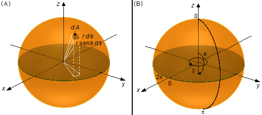
The limits of integration will be from 0 to π in dθ and from 0 and 2π in dϕ one lap at the base of the hemisphere, (Figure 3-B)

\[ Er^{2}\int_{0}^{\pi}\sin \theta \;d\theta \int_{0}^{{2\pi}}d\phi =\frac{q}{\epsilon_{0}} \]

Integration of \( \displaystyle \int_{0}^{\pi}\sin \theta \;d\theta \)

\[ \begin{split} \int_{0}^{\pi}\sin \theta \;d\theta &\Rightarrow \left.-\cos\theta \;\right|_{\;0}^{\;\pi }\Rightarrow -(\cos \pi -\cos0)\Rightarrow\\ &\Rightarrow -(-1-1)\Rightarrow -(-2)= 2 \end{split} \]

Integration of \( \displaystyle \int_{0}^{2\pi}\;d\phi \)

\[ \int_{0}^{2\pi}\;d\phi \Rightarrow\left.\phi \;\right|_{\;0}^{\;2\pi}\Rightarrow2\pi-0=2\pi \]

\[ Er^{2}\times 2\times 2\pi =\frac{q}{\epsilon_{0}} \]

\[ \bbox[#FFCCCC,10px] {E=\frac{q}{4\pi \epsilon_{0}r^{2}}} \]

Fisicaexe - Physics Solved Problems by Elcio Brandani Mondadori is licensed under a Creative Commons Attribution-NonCommercial-ShareAlike 4.0 International License .