Solved Problem on Coulomb's Law and Electric Field
advertisement
A disk of radius a carries a uniformly distributed charge Q. Calculate the electric field
vector:
a) At a point P on the axis of symmetry perpendicular to the plane of the disk at a distance z from its center;
b) In the case that the radius a of the disk is much greater than the distance from the point P to the disk, a>>z.
a) At a point P on the axis of symmetry perpendicular to the plane of the disk at a distance z from its center;
b) In the case that the radius a of the disk is much greater than the distance from the point P to the disk, a>>z.

Problem data:
- Radius of the disk: a;
- Charge of the disk: Q;
- Distance to the point where we want the electric field: z.
The position vector r goes from an element of charge dq to point P where we want to calculate the electric field, the vector rq locates the charge element relative to the origin of the reference frame, and the vector rp locates point P (Figure 1-A).
\[
\begin{gather}
\mathbf{r}={\mathbf{r}}_{p}-{\mathbf{r}}_{q}
\end{gather}
\]
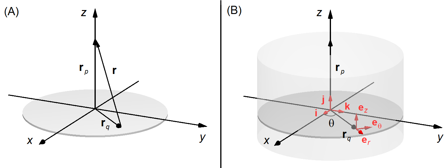
Based on the geometry of the problem, we choose cylindrical coordinates (Figure 1-B), the vector rq only has a component in the er direction, \( {\mathbf{r}}_{q}=r_{q}\;\mathbf{e}_{r} \) and the vector rp only has a component in the z direction, \( {\mathbf{r}}_{p}=r_{p}\;\mathbf{e}_{z} \). Converting cylindrical coordinates to Cartesian coordinates x, y and z are given by
\[
\begin{gather}
\left\{
\begin{array}{l}
x=r_{q}\cos \theta \\
y=r_{q}\operatorname{sen}\theta \\
z=z
\end{array}
\right. \tag{I}
\end{gather}
\]
Note: In the Figure 1-B, i, j e k are unit vectors in the Cartesian
coordinates, and er, eθ e
ez are unit vectors in the cylindrical coordinates.
After the conversion the vector rq, is written as \( {\mathbf{r}}_{q}=x\;\mathbf{i}+y\;\mathbf{j} \), and the vector rp as \( {\mathbf{r}}_{p}=z\;\mathbf{k} \).
The position vector will be
\[
\begin{gather}
\mathbf{r}=z\;\mathbf{k}-\left(x\;\mathbf{i}+y\;\mathbf{j}\right)\\[5pt]
\mathbf{r}=-x\;\mathbf{i}-y\;\mathbf{j}+z\;\mathbf{k} \tag{II}
\end{gather}
\]
From expression (II), the magnitude of the position vector r will be
\[
\begin{gather}
r^{2}=(-x)^{2}+(-y)^{2}+z^{2}\\[5pt]
r=\left(x^{2}+y^{2}+z^{2}\right)^{\frac{1}{2}} \tag{III}
\end{gather}
\]
Solution
a) The electric field vector is given by
\[
\begin{gather}
\bbox[#99CCFF,10px]
{\mathbf{E}=\frac{1}{4\pi \epsilon_{0}}\int{\frac{dq}{r^{2}}\;\frac{\mathbf{r}}{r}}}
\end{gather}
\]
\[
\begin{gather}
\mathbf{E}=\frac{1}{4\pi \epsilon_{0}}\int{\frac{dq}{r^{3}}\;\mathbf{r}} \tag{IV}
\end{gather}
\]
Using the expression of the surface density of charge σ, we have the charge element dq
\[
\begin{gather}
\bbox[#99CCFF,10px]
{\sigma =\frac{dq}{dA}}
\end{gather}
\]
\[
\begin{gather}
dq=\sigma \;dA \tag{V}
\end{gather}
\]
where dA is an element of area with angle dθ of the disk (Figure 2)
\[
\begin{gather}
dA=r_{q}\;dr_{q}\;d\theta \tag{VI}
\end{gather}
\]
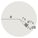
Figure 2
substituting the expression (VI) into expression (V)
\[
\begin{gather}
dq=\sigma r_{q}\;dr_{q}\;d\theta \tag{VII}
\end{gather}
\]
Substituting expressions (II), (III), and (VII) into expression (IV), and as the integration is made on the
surface of the disk, it depends on two variables rq and θ, we have a double integral
\[
\begin{gather}
\mathbf{E}=\frac{1}{4\pi \epsilon_{0}}\iint {\frac{\sigma r_{q}\;dr_{q}\;d\theta}{\left[\left(x^{2}+y^{2}+z^{2}\right)^{\frac{1}{2}}\right]^{3}}}\left(-x\;\mathbf{i}-y\;\mathbf{j}+z\;\mathbf{k}\right)\\[5pt]
\mathbf{E}=\frac{1}{4\pi \epsilon_{0}}\iint {\frac{\sigma r_{q}\;dr_{q}\;d\theta}{\left(x^{2}+y^{2}+z^{2}\right)^{\frac{3}{2}}}}\left(-x\;\mathbf{i}-y\;\mathbf{j}+z\;\mathbf{k}\right) \tag{VIII}
\end{gather}
\]
substituting expressions (I) into expression (VIII)
\[
\begin{gather}
\mathbf{E}=\frac{1}{4\pi \epsilon_{0}}\iint {\frac{\sigma r_{q}\;dr_{q}\;d\theta}{\left[\left(r_{q}\cos \theta\right)^{2}+\left(r_{q}\sin \theta\right)^{2}+z^{2}\right]^{\frac{3}{2}}}\left(-r_{q}\cos \theta\;\mathbf{i}-r_{q}\sin \theta\;\mathbf{j}+z\mathbf{k}\right)}\\[5pt]
\mathbf{E}=\frac{1}{4\pi\epsilon_{0}}\iint {\frac{\sigma r_{q}\;dr_{q}\;d\theta}{\left[r_{q}^{2}\cos ^{2}\theta +r_{q}^{2}\sin ^{2}\theta+z^{2}\right]^{\frac{3}{2}}}\left(-r_{q}\cos \theta\;\mathbf{i}-r_{q}\sin \theta\;\mathbf{j}+z\;\mathbf{k}\right)}\\[5pt]
\mathbf{E}=\frac{1}{4\pi\epsilon_{0}}\iint {\frac{\sigma r_{q}\;dr_{q}\;d\theta}{\left[r_{q}^{2}\underbrace{\left(\cos ^{2}\theta+\sin ^{2}\theta\right)}_{1}+z^{2}\right]^{\frac{3}{2}}}\left(-r_{q}\cos \theta\;\mathbf{i}-r_{q}\sin \theta\;\mathbf{j}+z\;\mathbf{k}\right)}\\[5pt]
\mathbf{E}=\frac{1}{4\pi\epsilon_{0}}\iint {\frac{\sigma r_{q}\;dr_{q}\;d\theta}{\left(r_{q}^{2}+z^{2}\right)^{\frac{3}{2}}}\left(-r_{q}\cos \theta\;\mathbf{i}-r_{q}\sin \theta\;\mathbf{j}+z\;\mathbf{k}\right)}
\end{gather}
\]
As the charge density σ is constant it is moved outside of the integral, and the integral of the sum
is equal to the sum of the integrals
\[
\begin{gather}
\mathbf{E}=\frac{\sigma}{4\pi \epsilon_{0}}\left(-\iint {\frac{r_{q}^{2}\cos \theta \;dr_{q}\;d\theta}{\left(r_{q}^{2}+z^{2}\right)^{\frac{3}{2}}}}\;\mathbf{i}-\iint {\frac{r_{q}^{2}\sin \theta\;dr_{q}\;d\theta}{\left(r_{q}^{2}+z^{2}\right)^{\frac{3}{2}}}}\;\mathbf{j}+z\iint {\frac{r_{q}\;dr_{q}\;d\theta}{\left(r_{q}^{2}+z^{2}\right)^{\frac{3}{2}}}}\;\mathbf{k}\right)
\end{gather}
\]
The limits of integration will be 0 and a in drq, along the disk radius, 0 and
2π in dθ, a complete lap in the ring, the integral can be separated
\[
\begin{split}
\mathbf{E} =\frac{\sigma}{4\pi \epsilon_{0}}\left(-\int_{0}^{a}{\frac{r_{q}^{2}\;dr_{q}}{\left(r_{q}^{2}+z^{2}\right)^{\frac{3}{2}}}}\underbrace{\int_{0}^{{2\pi}}{\cos \theta \;d\theta}}_{0}\;\mathbf{i} - \int_{0}^{a}{\frac{r_{q}^{2}\;dr_{q}}{\left(r_{q}^{2}+z^{2}\right)^{\frac{3}{2}}}}\underbrace{\int_{0}^{{2\pi}}{\sin \theta \;d\theta}}_{0}\;\mathbf{j}+\right.\\
\left.+z\int_{0}^{a}{\frac{r_{q}\;dr_{q}}{\left(r_{q}^{2}+z^{2}\right)^{\frac{3}{2}}}}\int_{0}^{{2\pi}}{d\theta }\;\mathbf{k}\right)
\end{split}
\]
Integration of \( \displaystyle \int_{0}^{{2\pi}}\cos \theta \;d\theta \)
1st method
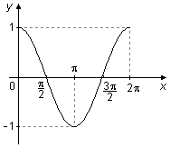 Figure 3
1st method
\[
\begin{align}
\int_{0}^{{2\pi}}\cos \theta \;d\theta &=\left.\sin \theta\;\right|_{\;0}^{\;2\pi }=\sin 2\pi-\sin 0=\\
&=0-0=0
\end{align}
\]
2nd method
The graph of cosine between 0 and 2π, has a "positive" area above the x-axis between 0 and \( \frac{\pi }{2} \) and between \( \frac{3\pi }{2} \) and 2π, and a "negative" area below the x-axis between \( \frac{\pi }{2} \) and \( \frac{3\pi }{2} \), these two areas cancel in the integration and the integral is equal to zero (Figure 3).
The graph of cosine between 0 and 2π, has a "positive" area above the x-axis between 0 and \( \frac{\pi }{2} \) and between \( \frac{3\pi }{2} \) and 2π, and a "negative" area below the x-axis between \( \frac{\pi }{2} \) and \( \frac{3\pi }{2} \), these two areas cancel in the integration and the integral is equal to zero (Figure 3).
Integration of \( \displaystyle \int_{0}^{{2\pi}}\sin \theta \;d\theta \)
1st method
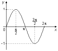 Figure 4
Figure 5
1st method
\[
\begin{align}
\int_{0}^{{2\pi}}\sin \theta \;d\theta &=\left.-\cos\theta \;\right|_{\;0}^{\;2\pi }=-(\cos 2\pi -\cos 0)=\\
&=-(1-1)=0
\end{align}
\]
2nd method
The graph of sine between 0 and 2π, has a "positive" area above the x-axis between 0 and π and a "negative" area below the x-axis between π and 2π, these two areas cancel in the integration and the integral is equal to zero (Figure 4).
The graph of sine between 0 and 2π, has a "positive" area above the x-axis between 0 and π and a "negative" area below the x-axis between π and 2π, these two areas cancel in the integration and the integral is equal to zero (Figure 4).
Note: The two integrals, in directions i and j which are zero, represent
the mathematical calculation for the assertion that is usually done that the components of the
electric field parallel to the xy plane, dEP, cancel. Only
normal components to the plane dEN contribute to the total electric
field (Figure 5).
Figure 5
Integration of \( \displaystyle \int_{0}^{a}{\frac{r_{q}\;dr_{q}}{\left(r_{q}^{2}+z^{2}\right)^{\frac{3}{2}}}} \)
Changing the variable
for rq = 0
we have \( u=0^{2}+z^{2}\Rightarrow u=z^{2} \)
for rq = a
we have \( u=a^{2}+z^{2} \)
Changing the variable
\[
\begin{array}{l}
u=r_{q}^{2}+z^{2}\\[5pt]
du=2r_{q}\;dr_{q}\Rightarrow dr_{q}=\dfrac{du}{2r_{q}}
\end{array}
\]
changing the limits of integration
for rq = 0
we have \( u=0^{2}+z^{2}\Rightarrow u=z^{2} \)
for rq = a
we have \( u=a^{2}+z^{2} \)
\[
\begin{align}
\int_{z^{2}}^{{a^{2}+z^{2}}}{\frac{r_{q}}{u^{\frac{3}{2}}}\;\frac{du}{2r_{q}}} &\Rightarrow\frac{1}{2}\int_{z^{2}}^{{a^{2}+z^{2}}}{\frac{1}{u^{\frac{3}{2}}}\;du}\Rightarrow\frac{1}{2}\left.\frac{u^{-{\frac{3}{2}+1}}}{-{\dfrac{3}{2}+1}}\;\right|_{\;z^{2}}^{\;a^{2}+z^{2}}\Rightarrow \\[5pt]
&\Rightarrow\frac{1}{2}\left.\frac{u^{\frac{-3+2}{2}}}{\dfrac{-{3+2}}{2}}\;\right|_{\;z^{2}}^{\;a^{2}+z^{2}}\Rightarrow\frac{1}{2}\left.\frac{u^{-{\frac{1}{2}}}}{-{\dfrac{1}{2}}}\;\right|_{\;z^{2}}^{\;a^{2}+z^{2}}\Rightarrow\\[5pt]
&\Rightarrow\ \left.-u^{-{\frac{1}{2}}}\;\right|_{\;z^{2}}^{\;a^{2}+z^{2}}\Rightarrow\left.-{\frac{1}{u^{\frac{1}{2}}}}\;\right|_{\;z^{2}}^{\;a^{2}+z^{2}}\Rightarrow \\[5pt]
&\Rightarrow-\left(\frac{1}{\sqrt{a^{2}+z^{2}}}-\frac{1}{\sqrt{z^{2}}}\right)\Rightarrow\frac{1}{z}-\frac{1}{\sqrt{a^{2}+z^{2}}}
\end{align}
\]
Integration of \( \displaystyle \int_{0}^{{2\pi}}d\theta \)
\[
\begin{gather}
\int_{0}^{{2\pi}} d\theta =\left.\theta\;\right|_{\;0}^{\;2\pi }=2\pi-0=2\pi
\end{gather}
\]
\[
\begin{gather}
\mathbf{E}=\frac{\sigma}{4\pi \epsilon_{0}}\left[0\;\mathbf{i}-0\;\mathbf{j}+z\;\left(\frac{1}{z}-\frac{1}{\sqrt{a^{2}+z^{2}}}\right)2\pi\;\mathbf{k}\right]\\[5pt]
\mathbf{E}=\frac{\sigma}{4\pi \epsilon_{0}}\left(\frac{z}{z}-\frac{z}{\sqrt{a^{2}+z^{2}}}\right)2\pi\;\mathbf{k}
\end{gather}
\]
\[
\begin{gather}
\bbox[#FFCCCC,10px]
{\mathbf{E}=\frac{\sigma}{2\epsilon_{0}}\left(1-\frac{z}{\sqrt{a^{2}+z^{2}\;}}\right)\;\mathbf{k}}
\end{gather}
\]
Figure 6
b) Letting the radius of the disk tend to the infinity (\( a\rightarrow \infty \))
\[
\begin{gather}
\mathbf{E}=\underset{a\rightarrow\infty }{\lim }{\frac{\sigma}{2\epsilon_{0}}}\left(1-\frac{z}{\sqrt{a^{2}+z^{2}}}\right)\;\mathbf{k}\\[5pt]
\mathbf{E}=\underset{a\rightarrow\infty }{\lim }\left[\frac{\sigma}{2\epsilon_{0}}-\frac{\sigma}{2\epsilon_{0}}\frac{z}{\sqrt{z^{2}\left(\dfrac{a^{2}}{z^{2}}+1\;\right)}}\right]\;\mathbf{k}\\[5pt]
\mathbf{E}=\underset{a\rightarrow\infty }{\lim }{\frac{\sigma}{2\epsilon_{0}}}\;\mathbf{k}-\underset{a\rightarrow\infty}\lim \left[{\;}\frac{\sigma}{2\epsilon_{0}}\frac{\cancel{z}}{\cancel{z}\sqrt{\left(\dfrac{a^{2}}{z^{2}}+1\;\right)}}\right]\;\mathbf{k}\\[5pt]
\mathbf{E}=\frac{\sigma}{2\epsilon_{0}}\;\mathbf{k}-\frac{\sigma}{2\epsilon_{0}}\underset{a\rightarrow \infty}{\lim}{\frac{1}{\sqrt{\left(\dfrac{a^{2}}{z^{2}}+1\;\right)}}\;\mathbf{k}}\\[5pt]
\mathbf{E}=\frac{\sigma}{2\epsilon_{0}}\;\mathbf{k}-\frac{\sigma}{2\epsilon_{0}}\frac{1}{\sqrt{\left(\dfrac{\infty^{2}}{z^{2}}+1\;\right)}}\;\mathbf{k}\\[5pt]
\mathbf{E}=\frac{\sigma}{2\epsilon_{0}}\;\mathbf{k}-\frac{\sigma}{2\epsilon_{0}}\frac{1}{\sqrt{\infty+1\;}}\;\mathbf{k}\\[5pt]
\mathbf{E}=\frac{\sigma}{2\epsilon_{0}}\;\mathbf{k}-\frac{\sigma}{2\epsilon_{0}}\frac{1}{\infty}\;\mathbf{k}\\[5pt]
\mathbf{E}=\frac{\sigma}{2\epsilon_{0}}\;\mathbf{k}-\frac{\sigma}{2\epsilon_{0}}.0\;\mathbf{k}
\end{gather}
\]
\[
\begin{gather}
\bbox[#FFCCCC,10px]
{\mathbf{E}=\frac{\sigma}{2\epsilon_{0}}\;\mathbf{k}}
\end{gather}
\]
Note: When we say "infinite radius" this does not mean that the plate is actually
infinite, but that the region considered is far from the edges of the board where the field is not
uniform due to the edge effects (Figure 7). In the region considered the value of the field is
constant.

advertisement

Fisicaexe - Physics Solved Problems by Elcio Brandani Mondadori is licensed under a Creative Commons Attribution-NonCommercial-ShareAlike 4.0 International License .