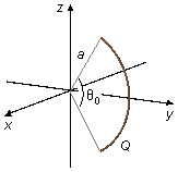
An arc of a circle of radius a and central angle θ0 carries an electric charge
Q uniformly distributed along the arc. Determine:
a) The electric field vector, at the points of the line passing through the center of the arc, and is
perpendicular to the plane containing the arc;
b) The electric field vector in the center of curvature of the arc;
c) The electric field vector when the central angle tends to zero.
Problem data:
- Radius of the arc: a;
- Central angle of the arc: θ0;
- Electric charge on the arc: Q.
Problem diagram:
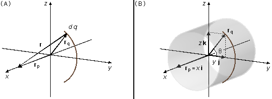
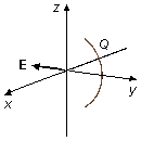
The position vector r goes from an element of charge dq to point P, where we want to
calculate the electric field, the vector rq locates the charge element relative to
the origin of the reference frame, and the vector rp locates point P
(Figure 1-A).
\[
\begin{gather}
\mathbf r=\mathbf r_p-\mathbf r_q
\end{gather}
\]
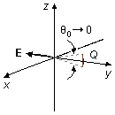
From the geometry of the problem, we choose cylindrical coordinates (Figure 1-B). The
rq vector, which is on the yz plane, is written as
\( \mathbf r_q=y\;\mathbf j+z\;\mathbf k \)
and the rp vector only has a component in the i direction,
\( \mathbf r_p=x\;\mathbf i \)
(contrary to what is usual, where the rq vector is on the xy plane and the
axis of the cylinder is in the k direction), the position vector will be
\[
\begin{gather}
\mathbf r=x\;\mathbf i-\left(y\;\mathbf j+z\;\mathbf k\right)\\[5pt]
\mathbf r=x\;\mathbf i-y\;\mathbf j-z\;\mathbf k \tag{I}
\end{gather}
\]
From equation (I), the magnitude of the position vector will be
\[
\begin{gather}
r^2=x^2+(-y)^2+(-z)^2\\[5pt]
r=\left(x^2+y^2+z^2\right)^{\frac{1}{2}} \tag{II}
\end{gather}
\]
where x, y, and z, in cylindrical coordinates, are given by
\[
\begin{gather}
\left\{
\begin{array}{l}
x=x\\
y=a\cos\theta\\
z=a\sin\theta
\end{array}
\right. \tag{III}
\end{gather}
\]
Solution:
a) The electric field vector is given by
\[
\begin{gather}
\bbox[#99CCFF,10px]
{\mathbf E=\frac{1}{4\pi\epsilon_0}\int{\frac{dq}{r^2}\;\frac{\mathbf r}{r}}}
\end{gather}
\]
\[
\begin{gather}
\mathbf E=\frac{1}{4\pi\epsilon_0}\int{\frac{dq}{r^{3}}\;\mathbf r} \tag{IV}
\end{gather}
\]
Using the equation for the linear density charge λ, we have the charge element dq.
\[
\begin{gather}
\bbox[#99CCFF,10px]
{\lambda=\frac{dq}{ds}}
\end{gather}
\]
\[
\begin{gather}
dq=\lambda\;ds \tag{V}
\end{gather}
\]
where
ds is an arc element with angle
dθ (Figure 2).
\[
\begin{gather}
ds=a\;d\theta \tag{VI}
\end{gather}
\]
substituting the equation (VI) into equation (V).
\[
\begin{gather}
dq=\lambda a\;d\theta \tag{VII}
\end{gather}
\]
Substituting equations (I), (II), and (VII) into equation (IV).
\[
\begin{gather}
\mathbf E=\frac{1}{4\pi\epsilon_0}\int{\frac{\lambda a\;d\theta}{\left[\left(x^2+y^2+z^2\right)^{1/2}\right]^{\;3}}}\left(x\;\mathbf i-y\;\mathbf j-z\;\mathbf k\right)\\[5pt]
\mathbf E=\frac{1}{4\pi\epsilon_0}\int{\frac{\lambda a\;d\theta}{\left(x^2+y^2+z^2\right)^{3/2}}}\left(x\;\mathbf i-y\;\mathbf j-z\;\mathbf k\right) \tag{VIII}
\end{gather}
\]
substituting equations (III) into equation (VIII).
\[
\begin{gather}
\mathbf E=\frac{1}{4\pi\epsilon_0}\int{\frac{\lambda a\;d\theta}{\left[\;x^2+\left(a\cos\theta\right)^2+\left(a\sin\theta\right)^2\right]^{3/2}}}\left(x\;\mathbf i-a\cos\theta\;\mathbf j-a\sin\theta\;\mathbf k\right)\\[5pt]
\mathbf E=\frac{1}{4\pi\epsilon_0}\int{\frac{\lambda a\;d\theta}{\left[x^2+a^2\cos^2\theta +a^2\sin^2\theta\;\right]^{3/2} }}\left(x\;\mathbf i-a\cos\theta\;\mathbf j-a\sin\theta\;\mathbf k\right)\\[5pt]
\mathbf E=\frac{1}{4\pi\epsilon_0}\int{\frac{\lambda a\;d\theta}{\left[x^2+a^2\underbrace{\left(\cos^2\theta+\sin^2\theta\right)}_{1}\right]^{3/2}}\left(x\;\mathbf i-a\cos\theta\;\mathbf j-a\sin\theta\;\mathbf k\right)}\\[5pt]
\mathbf E=\frac{1}{4\pi\epsilon_0}\int{\frac{\lambda a\;d\theta}{\left(x^2+a^2\right)^{3/2}}\left(x\;\mathbf i-a\cos\theta\;\mathbf j-a\sin\theta\;\mathbf k\right)}
\end{gather}
\]
As the charge density λ and the radius a are constants, they are moved outside the
integral, and the integral of the sum is equal to the sum of the integrals.
\[
\begin{gather}
\mathbf E=\frac{1}{4\pi\epsilon_0}\frac{\lambda a}{\left(x^2+a^2\right)^{3/2}}\left(x\int d\theta\;\mathbf i-a\int \cos\theta d\theta\;\mathbf j-a\int \sin\theta\;d\theta\;\mathbf k\right)
\end{gather}
\]
As there is symmetry, we can divide the central angle
θ0 into two parts measuring
\( \frac{\theta_0}{2} \)
clockwise and
\( -{\frac{\theta_0}{2}} \)
counterclockwise (Figure 3), the integration limits will be
\( -{\frac{\theta_0}{2}} \)
and
\( \frac{\theta_0}{2} \).
\[
\begin{gather}
\mathbf E=\frac{1}{4\pi\epsilon_0}\frac{\lambda a}{\left(x^2+a^2\right)^{3/2}}\left(x\int_{-{\frac{\theta_0}{2}}}^{{\frac{\theta_0}{2}}}d\theta\;\mathbf i-a\int_{-{\frac{\theta_0}{2}}}^{{\frac{\theta_0}{2}}}\cos\theta\;d\theta\;\mathbf j-a\int_{-{\frac{\theta_0}{2}}}^{{\frac{\theta_0}{2}}}\sin\theta\;d\theta\;\mathbf k\right)
\end{gather}
\]
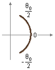
Figure 3
Integration of
\( \displaystyle \int_{-{\frac{\theta_0}{2}}}^{{\frac{\theta_0}{2}}}\;d\theta \)
\[
\begin{align}
\int_{-{\frac{\theta_0}{2}}}^{{\frac{\theta_0}{2}}}\;d\theta &=\frac{\theta_0}{2}-\left(-{\frac{\theta_0}{2}}\right)=\\
&=\frac{\theta_0}{2}+\frac{\theta_0}{2}=\cancel 2\frac{\theta_0}{\cancel 2}=\theta_0
\end{align}
\]
Integration of
\( \displaystyle \int_{-{\frac{\theta_{\;0}}{2}}}^{{\frac{\theta_{\;0}}{2}}}\cos\theta \;d\theta \)
\[
\begin{align}
\int_{-{\frac{\theta_0}{2}}}^{{\frac{\theta_0}{2}}}\cos\theta\;d\theta &=\left.\sin\theta\right|_{\;-\frac{\theta_0}{2}}^{\;\frac{\theta_0}{2}}=\\
&=\sin\frac{\theta_0}{2}-\sin\;\left(-{\frac{\theta_0}{2}}\right)
\end{align}
\]
the function sine is an odd function
\( f(-x)=-f(x) \),
\( \sin\left(-{\dfrac{\theta_0}{2}}\right)=-\sin\dfrac{\theta_0}{2} \)
\[
\begin{align}
\int_{-{\frac{\theta_0}{2}}}^{{\frac{\theta_0}{2}}}\cos\theta\;d\theta &=\sin\frac{\theta_0}{2}-\left[-\sin\;\frac{\theta_0}{2}\right]=\\
&=\sin\frac{\theta_0}{2}+\sin\frac{\theta_0}{2}=2\;\sin\;\frac{\theta_0}{2}
\end{align}
\]
Integration of
\( \displaystyle \int_{-{\frac{\theta_{;0}}{2}}}^{{\frac{\theta_{\;0}}{2}}}\sin\theta\;d\theta \)
\[
\begin{align}
\int_{-{\frac{\theta_0}{2}}}^{{\frac{\theta_0}{2}}}\sin\theta\;d\theta &=\left.-\cos\theta\right|_{\;-\frac{\theta_0}{2}}^{\;\frac{\theta_0}{2}}=\\
&=-\left[\cos\frac{\theta_0}{2}-\cos\left(-{\frac{\theta_0}{2}}\right)\right]
\end{align}
\]
the function cosine is an even function
\( f(x)=f(-x) \),
\( \cos\left(-{\dfrac{\theta_0}{2}}\right)=\cos\dfrac{\theta_0}{2} \)
\[
\begin{gather}
\int_{-{\frac{\theta_0}{2}}}^{{\frac{\theta_0}{2}}}\sin\theta\;d\theta=-\left[\cos\frac{\theta_0}{2}-\cos\frac{\theta_0}{2}\right]=0
\end{gather}
\]
\[
\begin{gather}
\mathbf E=\frac{1}{4\pi\epsilon_0}\frac{\lambda a}{\left(x^2+a^2\right)^{3/2}}\left(x\theta_0\;\mathbf i-2a\sin\frac{\theta_0}{2}\;\mathbf j-0\;\mathbf k\right)\\[5pt]
\mathbf E=\frac{1}{4\pi\epsilon_0}\frac{\lambda a}{\left(x^2+a^2\right)^{3/2}}\left(x\theta_0\;\mathbf i-2a\sin\frac{\theta_0}{2}\;\mathbf j\right) \tag{IX}
\end{gather}
\]
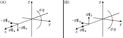
Note: The integral in the
k direction is equal to zero, because an element of charge
dq, produces at a point, an element of the field that can be decomposed into the elements,
dEx, −
dEy, and
−
dEz (Figure 4-A). Another element of charge placed in a symmetrical
position produces at the same point another element of the field that can be decomposed into the elements
dEx, −
dEy, and
dEz (Figure 4-B). Hence, the elements in the
k direction cancel, and
only elements in the
i and
j directions contribute to the total field.
The total charge of the arc is Q, and its length is aθ0, so the linear
density of charge can be written
\[
\begin{gather}
\lambda=\frac{Q}{a\theta_0} \tag{X}
\end{gather}
\]
substituting equation (X) into equation (IX).
\[
\begin{gather}
\mathbf E=\frac{1}{4\pi\epsilon_0}\frac{Q}{a\theta_0}\frac{a}{\left(x^2+a^2\right)^{3/2}}\left(x\theta_0\;\mathbf i-2a\sin\frac{\theta_0}{2}\;\mathbf j\right)\\[5pt]
\mathbf E=\frac{1}{4\pi\epsilon_0}\frac{Q}{\left(x^2+a^2\right)^{3/2}}\left(\frac{1}{\theta_0}x\theta_0\;\mathbf i-\frac{1}{\theta_0}2a\sin\frac{\theta_0}{2}\;\mathbf j\right)
\end{gather}
\]
\[
\begin{gather}
\bbox[#FFCCCC,10px]
{\mathbf E=\frac{1}{4\pi\epsilon_0}\frac{Q}{\left(x^2+a^2\right)^{3/2}}\left(x\;\mathbf i-\frac{2a}{\theta_0}\sin\frac{\theta_0}{2}\;\mathbf j\right)}
\end{gather}
\]
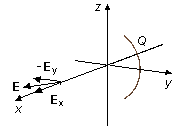
b) In the center of curvature, we have x = 0, substituting this in the solution of the previous item
(Figure 6).
\[
\begin{gather}
\mathbf E=\frac{1}{4\pi\epsilon_0}\frac{Q}{\left(0^2+a^2\right)^{3/2}}\left(0\;\mathbf i-\frac{2a}{\theta_0}\sin\frac{\theta_0}{2}\;\mathbf j\right)\\[5pt]
\mathbf E=\frac{-{1}}{4\pi\epsilon_0}\frac{Q}{a^{3}}\frac{2a}{\theta_0}\sin\frac{\theta_0}{2}\;\mathbf j
\end{gather}
\]
\[
\begin{gather}
\bbox[#FFCCCC,10px]
{\mathbf E=\frac{-{1}}{4\pi\epsilon_0}\frac{Q}{a^2}\frac{2}{\theta_0}\sin\frac{\theta_0}{2}\;\mathbf j}
\end{gather}
\]
c) When the central angle tends to zero
(\( \theta_0\rightarrow 0 \)),
the arc tends to a point charge, applying the limit to the solution of the previous item (Figure 7).
\[
\begin{gather}
\mathbf E=\underset{\theta_0\rightarrow0}{\lim}-\frac{1}{4\pi\epsilon_0}\;\frac{Q}{a^2}\frac{2}{\theta_0}\sin\frac{\theta_0}{2}\;\mathbf j
\end{gather}
\]
turning the term
\( \frac{2}{\theta_0} \)
upside down.
\[
\begin{gather}
\mathbf E=\underset{\theta_0\rightarrow 0}{\lim}-{\frac{1}{4\pi\epsilon_0}\frac{Q}{a^2}\dfrac{\sin\dfrac{\theta_0}{2}}{\dfrac{\theta_0}{2}}\;\mathbf j}
\end{gather}
\]
From the limit
\( \underset{x\rightarrow 0}{\lim}{\dfrac{\sin x}{x}}=1 \)
\[
\begin{gather}
\mathbf E=-{\frac{1}{4\pi\epsilon_0}}\frac{Q}{a^2}\underbrace{\;\underset{\theta_0\rightarrow 0}{\lim }{\dfrac{\sin\dfrac{\theta_0}{2}}{\dfrac{\theta_0}{2}}}}_{1}\;\mathbf j
\end{gather}
\]
\[
\begin{gather}
\bbox[#FFCCCC,10px]
{\mathbf E=-{\frac{Q}{4\pi\epsilon_0a^2}}\;\mathbf j}
\end{gather}
\]
and the result is reduced to the electric field vector of a point charge.