Solved Problem on Electric Field

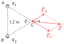
Two point charges of 5×10⁻⁶ C and 3×10⁻⁶ C, are placed in two vertices of an equilateral triangle with sides of 1.2 m. Calculate the magnitude of the electric field in the third vertex, assuming they are in the vacuum.

Problem data:

Charge 1: q₁ = 5×10⁻⁶ C;
Charge 2: q₂ = 3×10⁻⁶;
Distance between the charges: d = 1.2 m;
Coulomb Constant: \( k_e=9\times 10^9\;\mathrm{\frac{N.m^2}{C^2}} \).

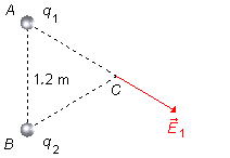
Construction of the resultant electric field vector:

Charges q₁ and q₂ are placed at vertices A and B of the triangle. Considering the charge q₁ of the highest value 5×10⁻⁶ C, we draw at point C the vector \( \vec E_1 \), in the direction of the segment \( \overline{AC} \), with the direction pointing away from the charge, q > 0. The highest value charge produces a more intense field (Figure 1).

Figure 1

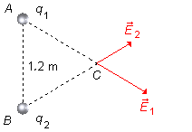
At point C we draw the vector \( \vec E_2 \), in the direction of segment \( \overline{BC} \), with direction away and smaller in size, the charge q₂ is smaller, 3×10⁻⁶ C, and produces a less intense field (Figure 2).

Figure 2

From the endpoint of vector \( \vec E_2 \) we draw a straight line parallel to the vector \( \vec E_1 \) (Figure 3).

Figure 3

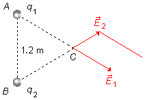
From the endpoint of vector \( \vec E_1 \) we draw a straight line parallel to the vector \( \vec E_2 \) (Figure 4).

Figure 4

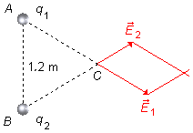
From vertex C to the intersection of the lines, we have the resultant vector \( \vec E \), where α is the angle between the electric field vectors \( \vec E_1 \) and \( \vec E_2 \). Since the triangle is equilateral, all its internal angles are equal to β = 60°. The angles α and β are vertically opposite angles, and the angle α is also 60° (Figure 5).

Figure 5

Solution:

The resultant electric field is given by

\[ \begin{gather} \vec E=\vec E_1+\vec E_2 \end{gather} \]

the magnitude can be calculated using the Law of Cosines

\[ \begin{gather} \bbox[#99CCFF,10px] {E^2=E_1^2+E_3^2+2E_1E_2\cos\alpha} \tag{I} \end{gather} \]

The magnitude of the electric field of each charge is calculated by

\[ \begin{gather} \bbox[#99CCFF,10px] {E=k_e\frac{q}{r^2}} \end{gather} \]

\[ \begin{gather} E_1=k_e\frac{q_1}{r_1^2}\\[5pt] E_1=\left(9\times 10^9\;\mathrm{\small{\frac{N.m^2}{C^{\cancel 2}}}}\right)\frac{5\times 10^{-6}\;\mathrm{\cancel C}}{(1.2\;\mathrm m)^2}\\[5pt] E_1=\frac{4.5\times 10^4\;\mathrm{\small{\frac{N.\cancel{m^2}}{C}}}}{1.44\;\mathrm{\cancel{m^2}}}\\[5pt] E_1\approx 3.1\times 10^4\;\mathrm{\frac{N}{C}} \tag{II} \end{gather} \]

\[ \begin{gather} E_2=k_e\frac{q_2}{r_2^2}\\[5pt] E_2=\left(9\times 10^9\;\mathrm{\small{\frac{N.m^2}{C^{\cancel 2}}}}\right)\frac{3\times 10^{-6}\;\mathrm{\cancel C}}{(1.2\;\mathrm m)^2}\\[5pt] E_2=\frac{2.7\times 10^4\;\mathrm{\small{\frac{N.\cancel{m^2}}{C}}}}{1.44\;\mathrm{\cancel{m^2}}}\\[5pt] E_2\approx 1.9\times 10^4\;\mathrm{\frac{N}{C}} \tag{III} \end{gather} \]

substituting equations (II) and (III) into equation (I)

\[ \begin{gather} E^2=\left(3.1\times 10^4\;\mathrm{\small{\frac{N}{C}}}\right)^2+\left(1.9\times 10^4\right)^2+2\times\left(3.1\times 10^4\;\mathrm{\small{\frac{N}{C}}}\right)\left(1.9\times 10^4\;\mathrm{\small{\frac{N}{C}}}\right)\cos60°\\[5pt] E^2=9.6\times 10^8\;\mathrm{\small{\left(\frac{N}{C}\right)^2}}+3.6\times 10^8\;\mathrm{\small{\left(\frac{N}{C}\right)^2}}+\cancel{2}\times 5.9\times 10^8\;\mathrm{\small{\left(\frac{N}{C}\right)^2}}\times\frac{1}{\cancel{2}}\\[5pt] E^2=(9.6+3.6+5.9)\times 10^8\;\mathrm{\small{\left(\frac{N}{C}\right)^2}}\\[5pt] E^2=19.1\times 10^8\;\mathrm{\small{\left(\frac{N}{C}\right)^2}}\\[5pt] E=\sqrt{19.1\times 10^8\;\mathrm{\small{\left(\frac{N}{C}\right)^2}}\;} \end{gather} \]

\[ \begin{gather} \bbox[#FFCCCC,10px] {E\approx 4.4\times 10^4\;\mathrm{\frac{N}{C}}} \end{gather} \]

Fisicaexe - Physics Solved Problems by Elcio Brandani Mondadori is licensed under a Creative Commons Attribution-NonCommercial-ShareAlike 4.0 International License .