Solved Problem on Coulomb's Law and Electric Field
advertisement
A square loop of side a carries a uniformly distributed charge Q. Determine the electric
field vector at points on the line perpendicular to the plane of the loop at a distance z from
its center.
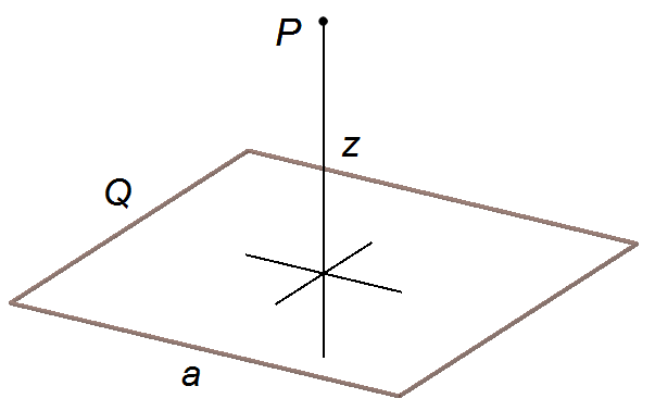
Problem data:
- Length of loop side: a;
- Distance to point P: z;
- Charge of the loop: Q.
Let's calculate the electric field produced by a segment of the loop that passes through point \( y=\frac{a}{2} \) and is parallel to the x-axis.
The position vector r goes from an element of charge dq of the loop to the point P where the electric field is to be calculated, the vector rq locates the element of charge dq relative to the origin of the reference frame and the vector rpP (Figure 1-A).
\[
\mathbf{r}={\mathbf{r}}_{p}-{\mathbf{r}}_{q}
\]

The vector rq is written as \( {\mathbf{r}}_{q}=x\;\mathbf{i}+y\;\mathbf{j} \) and the vector rp only has a component in the k direction, it is written as \( {\mathbf{r}}_{p}=z\;\mathbf{k} \) (Figure 1-B), and the position vector will be
\[
\begin{gather}
\mathbf{r}=z\;\mathbf{k}-(x\;\mathbf{i}+y\;\mathbf{j})\\
\mathbf{r}=-x\;\mathbf{i}-y\;\mathbf{j}+z\;\mathbf{k}\\
\mathbf{r}=-x\;\mathbf{i}-\frac{a}{2}\;\mathbf{j}+z\;\mathbf{k} \tag{I}
\end{gather}
\]
From expression (I) the magnitude of the position vector r will be
\[
\begin{gather}
r^{2}=x^{2}+\left(\frac{a}{2}\right)^{2}+z^{2}\\
r=\left[x^{2}+\left(\frac{a}{2}\right)^{2}+z^{2}\right]^{\;1/2}\\
r=\left(x^{2}+z^{2}+\frac{a^{2}}{4}\right)^{\;1/2} \tag{II}
\end{gather}
\]
Note: When the vector rq varies from
\( \frac{a}{2} \)
to
\( -{\frac{a}{2}} \),
(r1, r2, r3,...,
rn), the component of rq in the i direction
varies in magnitude (x1, x2, x3,...,
xn), but the component in the j direction is constant
\( \left(y=\frac{a}{2}\right) \).
This component goes from the origin to the wire on the y-axis (Figure 2).

Solution
The electric field vector is given by
\[ \bbox[#99CCFF,10px]
{\mathbf{E}=\frac{1}{4\pi\epsilon_{0}}\int{\frac{dq}{r^{2}}\;\frac{\mathbf{\text{r}}}{r}}}
\]
\[
\begin{gather}
{\mathbf{E}}_{1}=\frac{1}{4\pi \epsilon_{0}}\int{\frac{dq}{r^{3}}\;\mathbf{r}} \tag{III}
\end{gather}
\]
From the expression of the linear charge density λ, we obtain the charge element dq
\[ \bbox[#99CCFF,10px]
{\lambda =\frac{dq}{ds}}
\]
\[
\begin{gather}
dq=\lambda \;ds \tag{IV}
\end{gather}
\]
where ds is an element of wire length
\[
\begin{gather}
ds=dx \tag{V}
\end{gather}
\]
substituting expression (V) into expression (IV)
\[
\begin{gather}
dq=\lambda \;dx \tag{VI}
\end{gather}
\]
substituting expressions (I), (II), and (VI) into expression (III)
\[
\begin{gather}
{\mathbf{E}}_{1}=\frac{1}{4\pi \epsilon_{0}}\int {\frac{\lambda\;dx}{\left[\left(x^{2}+z^{2}+\dfrac{a^{2}}{4}\right)^{\;1/2}\right]^{3}}}\left(-x\;\mathbf{i}-\frac{a}{2}\;\mathbf{j}+z\;\mathbf{k}\right)\\[5pt]
{\mathbf{E}}_{1}=\frac{1}{4\pi\epsilon_{0}}\int {\frac{\lambda\;dx}{\left(x^{2}+z^{2}+\dfrac{a^{2}}{4}\right)^{\;3/2}}}\left(-x\;\mathbf{i}-\frac{a}{2}\;\mathbf{j}+z\;\mathbf{k}\right) \tag{VII}
\end{gather}
\]
Since the charge density λ is constant, the integral depends only on x, it can be moved out
of the integral
\[
{\mathbf{E}}_{1}=\frac{\lambda}{4\pi \epsilon_{0}}\int{\frac{dx}{\left(x^{2}+z^{2}+\dfrac{a^{2}}{4}\right)^{\;3/2}}}\left(-x\;\mathbf{i}-\frac{a}{2}\;\mathbf{j}+z\;\mathbf{k}\right)
\]
The integral will be done over all elements of length dx from
\( -{\frac{a}{2}} \)
to
\( \frac{a}{2} \)
(Figure 2)
\[
{\mathbf{E}}_{1}=\frac{\lambda}{4\pi \epsilon_{0}}\int_{{-a/2}}^{{a/2}}{\frac{dx}{\left(x^{2}+z^{2}+\dfrac{a^{2}}{4}\right)^{\;3/2}}}\left(-x\;\mathbf{i}-\frac{a}{2}\;\mathbf{j}+z\;\mathbf{k}\right)
\]
Using the Pythagorean Theorem, we obtain the distance h from the wire to the point
P (Figure 3)
\[
h^{2}=z^{2}+\frac{a^{2}}{4}
\]

\[
{\mathbf{E}}_{1}=\frac{\lambda}{4\pi \epsilon_{0}}\int_{{-a/2}}^{{a/2}}{\frac{dx}{\left(x^{2}+h^{2}\right)^{\;3/2}}}\left(-x\;\mathbf{i}-\frac{a}{2}\;\mathbf{j}+z\;\mathbf{k}\right)
\]
factoring h2 in the denominator and multiplying and dividing the expression by h
\[
\begin{gather}
{\mathbf{E}}_{1}=\frac{\lambda}{4\pi\epsilon_{0}}\int_{{-a/2}}^{{a/2}}{\frac{dx}{\left[h^{2}\left(\frac{x^{2}}{h^{2}}+1\right)\right]^{\;3/2}}}\left(-x\;\mathbf{i}-\frac{a}{2}\;\mathbf{j}+z\;\mathbf{k}\right)\times\frac{h}{h}\\[5pt]
{\mathbf{E}}_{1}=\frac{\lambda}{4\pi \epsilon_{0}}\int_{{-a/2}}^{{a/2}}{\frac{dx}{\left(h^{2}\right)^{3/2}\left[1+\left(\frac{x}{h}\right)^{2}\right]^{\;3/2}}}h\left(-{\frac{x}{h}}\;\mathbf{i}-\frac{a}{2h}\;\mathbf{j}+\frac{z}{h}\;\mathbf{k}\right)\\[5pt]
{\mathbf{E}}_{1}=\frac{\lambda}{4\pi \epsilon_{0}}\int_{{-a/2}}^{{a/2}}{\frac{dx}{h^{3}\left[1+\left(\frac{x}{h}\right)^{2}\right]^{\;3/2}}}h\left(-{\frac{x}{h}}\;\mathbf{i}-\frac{a}{2h}\;\mathbf{j}+\frac{z}{h}\;\mathbf{k}\right)\\[5pt]
{\mathbf{E}}_{1}=\frac{\lambda}{4\pi \epsilon_{0}}\int_{{-a/2}}^{{a/2}}{\frac{dx}{h^{2}\left[1+\left(\frac{x}{h}\right)^{2}\right]^{\;3/2}}}\left(-{\frac{x}{h}}\;\mathbf{i}-\frac{a}{2h}\;\mathbf{j}+\frac{z}{h}\;\mathbf{\text{k}}\right) \tag{VIII}
\end{gather}
\]
Considering the angle θ measured between h and the distance r, from the charge
element dq to the point P, the tangent of this angle will be (Figure 4)
\[
\begin{gather}
\tan \theta =\frac{x}{h} \tag{IX}
\end{gather}
\]
substituting expression (IX) into expression (VIII)

\[
\begin{gather}
{\mathbf{E}}_{1}=\frac{\lambda}{4\pi\epsilon_{0}}\int_{{-a/2}}^{{a/2}}{\frac{dx}{h^{2}\left[1+\left(\tan \theta\right)^{2}\right]^{\;3/2}}}\left(-{\tan \theta}\;\mathbf{i}-\frac{a}{2h}\;\mathbf{j}+\frac{z}{h}\;\mathbf{k}\right)\\[5pt]
{\mathbf{E}}_{1}=\frac{\lambda}{4\pi \epsilon_{0}}\int_{{-a/2}}^{{a/2}}{\frac{dx}{h^{2}\left[1+\tan ^{2}\theta\right]^{\;3/2}}}\left(-{\tan \theta}\;\mathbf{i}-\frac{a}{2h}\;\mathbf{j}+\frac{z}{h}\;\mathbf{\text{k}}\right) \tag{X}
\end{gather}
\]
From expression (IX), we obtain the element of length dx relative to the element of arc
dθ, changing the variable
\[
x=h\tan \theta
\]
Differentiation of
\( x=h\tan \theta \)
\[
\frac{dx}{d\theta}=h\frac{d}{d\theta}\left(\tan \theta \right)
\]
rewriting
\( \tan \theta=\dfrac{\sin \theta}{\cos \theta} \),
we have the differentiation of a quotient of functions given by the formula
\[
\left(\frac{u}{v}\right)^{\Large '}=\frac{u'v-u\;v'}{v^{2}}
\]
\[
\begin{align}
\frac{d}{d\theta}\left(\tan \theta \right)=\frac{d}{d\theta}\left(\frac{\sin \theta}{\cos \theta}\right) &=\frac{\cos\theta \cos \theta-\sin \theta (-\operatorname{sen}\theta)}{(\cos \theta)^{2}}=\\
&=\frac{\cos ^{2}\theta+\sin ^{2}\theta}{\cos ^{2}\theta}=\frac{1}{\cos^{2}\theta}
\end{align}
\]
\[
\begin{gather}
\frac{dx}{d\theta}=h\frac{1}{\cos ^{2}\theta}
\end{gather}
\]
Note: The books on Integral and Differential Calculus give the derivative of the
tangent in form
\( \left(\tan \theta \right)^{'}=\operatorname{sec}^{2}\theta \),
where
\( \operatorname{sec}\theta=\dfrac{1}{\cos \theta} \),
but here for reasons of further simplification, we will let the derivative in the form shown above.
\[
\begin{gather}
\frac{dx}{d\theta}=h\frac{1}{\cos ^{2}\theta} \tag{XI}
\end{gather}
\]
substituting the tangent with
\( \frac{\sin \theta}{\cos \theta} \)
and the expression (XI) into the expression(X)
\[
\begin{gather}
{\mathbf{E}}_{1}=\frac{\lambda}{4\pi\epsilon_{0}}\int_{{-a/2}}^{{a/2}}{\frac{1}{h^{2}\left[1+\left(\dfrac{\sin \theta}{\cos \theta}\right)^{2}\right]^{\;3/2}}}h\;\frac{d\theta}{\cos^{2}\theta}\left(-{\frac{\sin \theta}{\cos \theta}}\;\mathbf{i}-\frac{a}{2h}\;\mathbf{j}+\frac{z}{h}\;\mathbf{k}\right)\\[5pt]
{\mathbf{E}}_{1}=\frac{\lambda}{4\pi \epsilon_{0}}\int_{{-a/2}}^{{a/2}}{\frac{1}{h\left[1+\left(\dfrac{\sin \theta}{\cos\theta}\right)^{2}\right]^{\;3/2}}}\frac{d\theta}{\cos^{2}\theta }\left(-{\frac{\sin \theta}{\cos \theta}}\;\mathbf{i}-\frac{a}{2h}\;\mathbf{j}+\frac{z}{h}\;\mathbf{k}\right)
\end{gather}
\]
The limits of integration for the variable θ are −θm, the maximum
value measured counterclockwise, when x is
\( \frac{a}{2} \),
and θm, the maximum value measured clockwise, when x is
\( -{\frac{a}{2}} \)
(Figure 5).

Note: In Figure 5, it may seem inconsistent that for the side measuring
\( \frac{a}{2} \)
the angle is −θm, and for
\( -{\frac{a}{2}} \)
the angle is θm. This is due to the sign convention, angles are measured from the
h line, clockwise we have a positive angle, and counterclockwise we have a negative angle.
\[
\begin{gather}
{\mathbf{E}}_{1}=\frac{\lambda}{4\pi\epsilon_{0}}\int_{{-\theta_{m}}}^{{\theta_{m}}}{\frac{1}{h\left(1+\dfrac{\sin ^{2}\theta}{\cos^{2}\theta}\right)^{\;3/2}}}\frac{d\theta}{\cos ^{2}\theta}\left(-{\frac{\sin \theta}{\cos \theta}}\;\mathbf{i}-\frac{a}{2h}\;\mathbf{j}+\frac{z}{h}\;\mathbf{k}\right)\\[5pt]
{\mathbf{E}}_{1}=\frac{\lambda}{4\pi \epsilon_{0}}\int_{{-\theta_{m}}}^{{\theta_{m}}}{\frac{1}{h\left(\dfrac{\cos ^{2}+\sin ^{2}\theta}{\cos ^{2}\theta}\right)^{\;3/2}}}\frac{d\theta}{\cos ^{2}\theta}\left(-{\frac{\sin \theta}{\cos \theta}}\;\mathbf{i}-\frac{a}{2h}\;\mathbf{j}+\frac{z}{h}\;\mathbf{k}\right)\\[5pt]
{\mathbf{\text{E}}}_{1}=\frac{\lambda}{4\pi \epsilon_{0}}\int_{{-\theta_{m}}}^{{\theta_{m}}}{\frac{1}{h\dfrac{1}{\left(\cos ^{2}\theta\right)^{\;3/2}}}}\frac{d\theta}{\cos ^{2}\theta}\left(-{\frac{\sin \theta}{\cos \theta}}\;\mathbf{i}-\frac{a}{2h}\;\mathbf{j}+\frac{z}{h}\;\mathbf{k}\right)\\[5pt]
{\mathbf{E}}_{1}=\frac{\lambda}{4\pi \epsilon_{0}}\int_{{-\theta_{m}}}^{{\theta_{m}}}{\frac{1}{h\dfrac{1}{\cos ^{\cancel{3}}\theta }}}\frac{d\theta}{\cancel{\cos^{2}}\theta}\left(-{\frac{\sin \theta }{\cos \theta}}\;\mathbf{i}-\frac{a}{2h}\;\mathbf{j}+\frac{z}{h}\;\mathbf{k}\right)\\[5pt]
{\mathbf{E}}_{1}=\frac{\lambda}{4\pi \epsilon_{0}}\int_{{-\theta_{m}}}^{{\theta_{m}}}{\frac{1}{h\dfrac{1}{\cos \theta }}}d\theta\left(-{\frac{\sin \theta}{\cos \theta}}\;\mathbf{i}-\frac{a}{2k}\;\mathbf{j}+\frac{z}{k}\;\mathbf{k}\right)\\[5pt]
{\mathbf{E}}_{1}=\frac{\lambda}{4\pi \epsilon _{0}}\int_{{-\theta_{m}}}^{{\theta_{m}}}{\frac{\cos\theta}{h}}d\theta \left(-{\frac{\sin \theta}{\cos\theta}}\;\mathbf{i}-\frac{a}{2h}\;\mathbf{j}+\frac{z}{h}\;\mathbf{k}\right)
\end{gather}
\]
Since h, a, and z are constants, the integral depends only on θ, they can be
moved out of the integral, and the integral of the sum of functions equal to the sum of the integrals
\[
\begin{gather}
{\mathbf{E}}_{1}=\frac{\lambda}{4\pi\epsilon_{0}h}\left(-\int_{{-\theta_{m}}}^{{\theta_{m}}}{\cos\theta}\frac{\sin \theta}{\cos \theta}\;d\theta\;\mathbf{i}-\int_{{-\theta_{m}}}^{{\theta_{m}}}{\cos\theta }\frac{a}{2h}\;d\theta \;\mathbf{j}+\int_{{-\theta_{m}}}^{{\theta_{m}}}{\cos \theta}\frac{z}{h}\;d\theta\;\mathbf{k}\right)\\[5pt]
{\mathbf{E}}_{1}=\frac{\lambda}{4\pi \epsilon_{0}h}\left(\underbrace{-\int_{{-\theta_{m}}}^{{\theta_{m}}}{\sin \theta}\;d\theta\;\mathbf{i}}_{0}-\frac{a}{2h}\int_{{-\theta_{m}}}^{{\theta_{m}}}{\cos \theta}\;d\theta\;\mathbf{j}+\frac{z}{h}\int_{{-\theta_{m}}}^{{\theta_{m}}}{\cos \theta}\;d\theta\;\mathbf{k}\right)
\end{gather}
\]
Integration of \( \displaystyle \int_{{-\theta_{m}}}^{{\theta_{m}}}\cos \theta \;d\theta \)
1st method
Since the cosine function is an even function, f(x) = f(−x), we can integrate over half the range (from 0 to θm) and multiply the integral by 2
We can integrate over the whole interval (from −θm to θm)
1st method
Since the cosine function is an even function, f(x) = f(−x), we can integrate over half the range (from 0 to θm) and multiply the integral by 2
\[
2\int_{0}^{{\theta_{m}}}\cos \theta \;d\theta=2\left.\sin \theta \right|_{\;0}^{\;\theta_{m}}=2(\sin \theta_{m}-\operatorname{sen}0)=2(\sin \theta_{m}-0)=2\sin \theta_{m}
\]
2nd method
We can integrate over the whole interval (from −θm to θm)
\[
\int_{{-\theta_{m}}}^{{\theta_{m}}}\cos \theta \;d\theta=\left.\sin \theta \;\right|_{\;-\theta_{m}}^{\;\theta_{m}}=\sin \theta_{m}-\operatorname{sen}(-\theta_{m})
\]
Since sine is an odd function, f(−x) = −f(x), we have
\( \sin (-\theta_{m})=-\sin (\theta_{m}) \)
\[
\int_{{-\theta_{m}}}^{{\theta_{m}}}\cos \theta \;d\theta=\sin \theta _{m}-(-\sin \theta_{m})=\operatorname{sen}\theta_{m}+\sin (\theta_{m})=2\sin \theta_{m}
\]
Integration of \( \displaystyle \int_{{-\theta_{m}}}^{{\theta_{m}}}\sin \theta \;d\theta \)
1st method

 Figure 6
1st method
\[
\int_{{-\theta_{m}}}^{{\theta_{m}}}\sin \theta \;d\theta=-\left.\cos \theta \;\right|_{\;-\theta_{m}}^{\;\theta_{m}}=-\left[\cos \theta_{m}-\cos (-\theta_{m})\right]
\]
since cosine is an even function, f(x) = f(−x), we have
\( \cos (\theta_{m})=\cos (-\theta_{m}) \)
\[
\int_{{-\theta_{m}}}^{{\theta_{m}}}\sin \theta \;d\theta=-(\cos \theta_{m}-\cos \theta_{m})=0
\]
2nd method
The graph of sine between −θm and 0 has a "negative" area below the
x-axis, and between 0 and θm a "positive" area above the x-axis
these two areas cancel each other out in the calculation of the integral, the value of the integral
equals zero in the i direction.
Note: The integral in the i direction, equal to zero, represents the mathematical
calculation for the assertion that is usually made, that the components of the electric field parallel
to the x-axis (E i and −E i) vanish. Only the components in
the j and k directions (−E j e E k) contribute to the
total electric field (Figure 6).
\[
\begin{gather}
{\mathbf{E}}_{1}=\frac{\lambda}{4\pi\epsilon_{0}h}\left(-0\;\mathbf{i}-\frac{a}{2h}2\sin \theta_{m}\;\mathbf{j}+\frac{z}{h}2\sin \theta_{m}\;\mathbf{k}\right)\\[5pt]
{\mathbf{E}}_{1}=\frac{\lambda}{4\pi \epsilon_{0}h^{2}}2\sin \theta_{m}\left(-{\frac{a}{2}}\;\mathbf{j}+z\;\mathbf{k}\right)\\[5pt]
{\mathbf{E}}_{1}=\frac{\lambda}{2\pi \epsilon_{0}h^{2}}\sin \theta_{m}\left(-{\frac{a}{2}}\;\mathbf{j}+z\;\mathbf{k}\right) \tag{XII}
\end{gather}
\]
The sine of θm can be obtained from Figure 7
\[
\begin{gather}
\sin \theta_{m}=\frac{\frac{a}{2}}{r}\\[5pt]
\sin \theta_{m}=\frac{a}{2r} \tag{XIII}
\end{gather}
\]

The hypotenuse r is given by the Pythagorean Theorem
\[
\begin{gather}
r^{2}=h^{2}+\left(\frac{a}{2}\right)^{2}\\r^{2}=h^{2}+\frac{a^{2}}{4}\\
r=\sqrt{h^{2}+\frac{a^{2}}{4}\;} \tag{XIV}
\end{gather}
\]
substituting expression (XIV) into expression (XIII)
\[
\begin{gather}
\sin \theta_{m}=\frac{a}{2\sqrt{h^{2}+\frac{a^{2}}{4}\;}} \tag{XV}
\end{gather}
\]
substituting expression (XV) into expression (XII) and the value of h2
\[
\begin{gather}
{\mathbf{\text{E}}}_{1}=\frac{\lambda}{2\pi\epsilon_{0}h^{2}}\frac{a}{2\sqrt{h^{2}+\dfrac{a^{2}}{4}\;}}\left(-{\frac{a}{2}}\;\mathbf{j}+z\;\mathbf{k}\right)\\[5pt]
{\mathbf{E}}_{1}=\frac{\lambda}{4\pi \epsilon_{0}\left(z^{2}+\dfrac{a^{2}}{4}\right)}\frac{a}{\sqrt{z^{2}+\dfrac{a^{2}}{4}+\dfrac{a^{2}}{4}\;}}\left(-{\frac{a}{2}}\;\mathbf{j}+z\;\mathbf{k}\right)
\end{gather}
\]
The electric field vector E1 has components in the j and k directions
(Figure 8)
\[
{\mathbf{E}}_{1}=\frac{\lambda}{4\pi \epsilon_{0}\left(z^{2}+\dfrac{a^{2}}{4}\right)}\frac{a}{\sqrt{z^{2}+\dfrac{a^{2}}{2}\;}}\left(-{\frac{a}{2}}\;\mathbf{j}+z\;\mathbf{k}\right)
\]

The other wire segments are symmetric, they will produce similar fields in different directions (Figure 9-A).
\[
{\mathbf{E}}_{2}=\frac{\lambda}{4\pi \epsilon_{0}\left(z^{2}+\dfrac{a^{2}}{4}\right)}\frac{a}{\sqrt{z^{2}+\dfrac{a^{2}}{2}\;}}\left(\frac{a}{2}\;\mathbf{j}+z\;\mathbf{k}\right)
\]
\[
{\mathbf{E}}_{3}=\frac{\lambda}{4\pi \epsilon_{0}\left(z^{2}+\dfrac{a^{2}}{4}\right)}\frac{a}{\sqrt{z^{2}+\dfrac{a^{2}}{2}\;}}\left(-{\frac{a}{2}}\;\mathbf{i}+z\;\mathbf{k}\right)
\]
\[
{\mathbf{E}}_{4}=\frac{\lambda}{4\pi \epsilon_{0}\left(z^{2}+\dfrac{a^{2}}{4}\right)}\frac{a}{\sqrt{z^{2}+\dfrac{a^{2}}{2}\;}}\left(\frac{a}{2}\;\mathbf{i}+z\;\mathbf{k}\right)
\]
The total electric field vector will be given by the sum of the electric field vectors produced by the four
sides (Figure 9-B)

\[
\begin{split}
\mathbf{E} &=\frac{\lambda}{4\pi\epsilon_{0}\left(z^{2}+\dfrac{a^{2}}{4}\right)}\frac{a}{\sqrt{z^{2}+\dfrac{a^{2}}{2}\;}}\left(-{\frac{a}{2}}\;\mathbf{j}+z\;\mathbf{k}\right)+\\[5pt]
&+\frac{\lambda}{4\pi\epsilon_{0}\left(z^{2}+\dfrac{a^{2}}{4}\right)}\frac{a}{\sqrt{z^{2}+\dfrac{a^{2}}{2}\;}}\left(\frac{a}{2}\;\mathbf{j}+z\;\mathbf{k}\right)+\\[5pt]
&+\frac{\lambda}{4\pi\epsilon_{0}\left(z^{2}+\dfrac{a^{2}}{4}\right)}\frac{a}{\sqrt{z^{2}+\dfrac{a^{2}}{2}\;}}\left(-{\frac{a}{2}}\;\mathbf{i}+z\;\mathbf{k}\right)+\\[5pt]
&+\frac{\lambda}{4\pi\epsilon_{0}\left(z^{2}+\frac{a^{2}}{4}\right)}\frac{a}{\sqrt{z^{2}+\frac{a^{2}}{2}\;}}\left(\frac{a}{2}\;\mathbf{i}+z\;\mathbf{k}\right)\\[5pt]
\mathbf{E} &=\frac{\lambda}{4\pi\epsilon_{0}\left(z^{2}+\dfrac{a^{2}}{4}\right)}\frac{a}{\sqrt{z^{2}+\dfrac{a^{2}}{2}\;}}\times{}\\[5pt]
&\times\left(-{\frac{a}{2}}\;\mathbf{j}+z\;\mathbf{k}\right)+\left(\frac{a}{2}\;\mathbf{j}+z\;\mathbf{k}\right)+\left(-{\frac{a}{2}}\;\mathbf{i}+z\;\mathbf{k}\right)+\left(\frac{a}{2}\;\mathbf{i}+z\;\mathbf{k}\right)\\[5pt]
\mathbf{E} &=\frac{\lambda}{4\pi\epsilon_{0}\left(z^{2}+\dfrac{a^{2}}{4}\right)}\frac{a}{\sqrt{z^{2}+\dfrac{a^{2}}{2}\;}}\times{}\\[5pt]
&\times\left(-{\frac{a}{2}}\;\mathbf{j}+z\;\mathbf{k}+\frac{a}{2}\;\mathbf{j}+z\;\mathbf{k}-\frac{a}{2}\;\mathbf{i}+z\;\mathbf{k}+\frac{a}{2}\;\mathbf{i}+z\;\mathbf{k}\right)\\[5pt]
\mathbf{E} &=\frac{\lambda}{4\pi \epsilon_{0}\left(z^{2}+\dfrac{a^{2}}{4}\right)}\frac{a}{\sqrt{z^{2}+\dfrac{a^{2}}{2}\;}}4z\;\mathbf{k}
\end{split}
\]
\[ \bbox[#FFCCCC,10px]
{\mathbf{E}=\frac{4\lambda az}{4\pi \epsilon_{0}\left(z^{2}+\dfrac{a^{2}}{4}\right)\sqrt{z^{2}+\dfrac{a^{2}}{2}\;}}\;\mathbf{k}}
\]
Note: The calculations that give the expressions for the electric field vectors
E2, E3 and E4 are as follows:
 Figure 10
The integrals will be
Figure 10
The integrals will be
 Figure 11
The integrals will be
Figure 11
The integrals will be
 Figure 12
The integrals will be
Figure 12
The integrals will be
The electric field produced by a segment of the loop that passes through the point
\( y=-{\frac{a}{2}} \)
and is parallel to the x-axis (Figure 10).
The vector rq will be \( {\mathbf{r}}_{q}=x\;\mathbf{i}-y\;\mathbf{j} \) and the vector rp will be \( {\mathbf{r}}_{p}=z\;\mathbf{k} \).
The vector r will be \( \mathbf{r}=-x\;\mathbf{i}+\frac{a}{2}\;\mathbf{j}+z\;\mathbf{k} \).
The electric field will be
The vector rq will be \( {\mathbf{r}}_{q}=x\;\mathbf{i}-y\;\mathbf{j} \) and the vector rp will be \( {\mathbf{r}}_{p}=z\;\mathbf{k} \).
The vector r will be \( \mathbf{r}=-x\;\mathbf{i}+\frac{a}{2}\;\mathbf{j}+z\;\mathbf{k} \).
The electric field will be
\[
{\mathbf{E}}_{2}=\frac{\lambda}{4\pi \epsilon_{0}}\int_{{-a/2}}^{{a/2}}{\frac{dx}{\left(x^{2}+z^{2}+\dfrac{a^{2}}{4}\right)^{\;3/2}}}\left(-x\;\mathbf{i}+\frac{a}{2}\;\mathbf{j}+z\;\mathbf{k}\right)
\]
\[
{\mathbf{E}}_{2}=\frac{\lambda}{4\pi \epsilon_{0}h}\left(\underbrace{-\int_{{-\theta_{m}}}^{{\theta_{m}}}{\sin \theta}\;d\theta\;\mathbf{i}}_{0}+\frac{a}{2h}\int_{{-\theta_{m}}}^{{\theta_{m}}}{\cos \theta}\;d\theta\;\mathbf{j}+\frac{z}{h}\int_{{-\theta_{m}}}^{{\theta_{m}}}{\cos \theta }\;d\theta \;\mathbf{k}\right)
\]
After integration
\[
{\mathbf{E}}_{2}=\frac{\lambda}{2\pi \epsilon_{0}h^{2}}\sin \theta_{m}\left(\frac{a}{2}\;\mathbf{j}+z\;\mathbf{k}\right)
\]
After the same calculations for the determination of sin θm
\[
{\mathbf{E}}_{2}=\frac{\lambda}{4\pi \epsilon_{0}\left(z^{2}+\dfrac{a^{2}}{4}\right)}\frac{a}{\sqrt{z^{2}+\dfrac{a^{2}}{2}\;}}\left(\frac{a}{2}\;\mathbf{j}+z\;\mathbf{k}\right)
\]
The electric field produced by a segment of the loop that passes through the point
\( x=\frac{a}{2} \)
and is parallel to the x-axis (Figure 11).
The vector rq will be \( {\mathbf{r}}_{q}=x\;\mathbf{i}-y\;\mathbf{j} \) and the vector rp will be \( {\mathbf{r}}_{p}=z\;\mathbf{k} \).
The vector r will be \( \mathbf{r}=-{\frac{a}{2}}\;\mathbf{i}+y\;\mathbf{j}+z\;\mathbf{k} \).
The electric field will be
The vector rq will be \( {\mathbf{r}}_{q}=x\;\mathbf{i}-y\;\mathbf{j} \) and the vector rp will be \( {\mathbf{r}}_{p}=z\;\mathbf{k} \).
The vector r will be \( \mathbf{r}=-{\frac{a}{2}}\;\mathbf{i}+y\;\mathbf{j}+z\;\mathbf{k} \).
The electric field will be
\[
{\mathbf{E}}_{3}=\frac{\lambda }{4\pi \epsilon_{0}}\int_{{-a/2}}^{{a/2}}{\frac{dy}{\left(y^{2}+z^{2}+\dfrac{a^{2}}{4}\right)^{\;3/2}}}\left(-{\frac{a}{2}}\;\mathbf{i}+y\;\mathbf{j}+z\;\mathbf{k}\right)
\]
\[
{\mathbf{E}}_{3}=\frac{\lambda}{4\pi \epsilon_{0}h}\left(-{\frac{a}{2h}}\int_{{-\theta_{m}}}^{{\theta_{m}}}{\cos\theta}\;d\theta \;\mathbf{i}\underbrace{+\int_{{-\theta_{m}}}^{{\theta_{m}}}{\sin \theta}\;d\theta}_{0}+\;\mathbf{j}+\frac{z}{h}\int_{{-\theta_{m}}}^{{\theta_{m}}}{\cos \theta}\;d\theta\;\mathbf{k}\right)
\]
After integration
\[
{\mathbf{E}}_{3}=\frac{\lambda}{2\pi \epsilon_{0}h^{2}}\sin \theta_{m}\left(-{\frac{a}{2}}\;\mathbf{j}+z\;\mathbf{k}\right)
\]
After the same calculations for the determination of sin θm
\[
{\mathbf{E}}_{3}=\frac{\lambda}{4\pi \epsilon_{0}\left(z^{2}+\dfrac{a^{2}}{4}\right)}\frac{a}{\sqrt{z^{2}+\dfrac{a^{2}}{2}\;}}\left(-{\frac{a}{2}}\;\mathbf{j}+z\;\mathbf{k}\right)
\]
The electric field produced by a segment of the loop that passes through the point
\( x=-{\frac{a}{2}} \)
and is parallel to the x-axis (Figure 12).
The vector rq will be \( {\mathbf{r}}_{q}=-x\;\mathbf{i}+y\;\mathbf{j} \) and the vector rp will be \( {\mathbf{r}}_{p}=z\;\mathbf{k} \).
The vector r will be \( \mathbf{r}=\frac{a}{2}\;\mathbf{i}-y\;\mathbf{j}+z\;\mathbf{k} \).
The electric field will be
The vector rq will be \( {\mathbf{r}}_{q}=-x\;\mathbf{i}+y\;\mathbf{j} \) and the vector rp will be \( {\mathbf{r}}_{p}=z\;\mathbf{k} \).
The vector r will be \( \mathbf{r}=\frac{a}{2}\;\mathbf{i}-y\;\mathbf{j}+z\;\mathbf{k} \).
The electric field will be
\[
{\mathbf{E}}_{3}=\frac{\lambda}{4\pi \epsilon_{0}}\int_{{-a/2}}^{{a/2}}{\frac{dy}{\left(y^{2}+z^{2}+\dfrac{a^{2}}{4}\right)^{\;3/2}}}\left(\frac{a}{2}\;\mathbf{i}-y\;\mathbf{j}+z\;\mathbf{k}\right)
\]
\[
{\mathbf{E}}_{4}=\frac{\lambda}{4\pi \epsilon_{0}h}\left(\frac{a}{2h}\int_{{-\theta_{m}}}^{{\theta_{m}}}{\cos\theta}\;d\theta \;\mathbf{i}\underbrace{-\int_{{-\theta_{m}}}^{{\theta_{m}}}{\sin \theta}\;d\theta}_{0}+\;\mathbf{\text{j}}+\frac{z}{h}\int_{{-\theta_{m}}}^{{\theta_{m}}}{\cos \theta}\;d\theta\;\mathbf{k}\right)
\]
After integration
\[
{\mathbf{E}}_{4}=\frac{\lambda}{2\pi \epsilon_{0}h^{2}}\sin \theta_{m}\left(\frac{a}{2}\;\mathbf{j}+z\;\mathbf{k}\right)
\]
After the same calculations for the determination of sin θm
\[
{\mathbf{E}}_{4}=\frac{\lambda}{4\pi \epsilon_{0}\left(z^{2}+\dfrac{a^{2}}{4}\right)}\frac{a}{\sqrt{z^{2}+\dfrac{a^{2}}{2}\;}}\left(\frac{a}{2}\;\mathbf{j}+z\;\mathbf{k}\right)
\]
advertisement

Fisicaexe - Physics Solved Problems by Elcio Brandani Mondadori is licensed under a Creative Commons Attribution-NonCommercial-ShareAlike 4.0 International License .