Solved Problem on Coulomb's Law and Electric Field

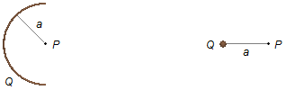
A wire is folded in a semicircular form of radius a, this wire carries a uniformly distributed charge Q. At point P, in the center of the semicircle, this distribution of charges produces an electric field of magnitude E₁.
If the wire is substituted by a point charge of the same value Q and at a distance a, equal to the radius of the semicircle, from the point P it produces at this point an electric field of magnitude E₂.
Calculate the ratio E₁/E₂, between the magnitudes of the electric fields produced by semicircular charges and by the point charge.

Problem data:

Radius of the semicircle: a;
Charge of the semicircle: Q;
Point charge: Q.

Problem diagram:

The position vector r goes from an element of charge dq of the arc to point P where we want to calculate the electric field, the vector r_q locates the charge element relative to the origin of the reference frame, and the vector r_p locates point P, as in this case the point P is at the origin, the r_p vector is equal to zero, r_p = 0 (Figure 1-A).

\[ \mathbf{r}={\mathbf{r}}_{p}-{\mathbf{r}}_{q} \]

Figure 1

From the geometry of the problem, we choose polar coordinates (Figure 1-B), the r_q vector is written as \( {\mathbf{r}}_{q}=-x\;\mathbf{i}+y\;\mathbf{j} \), the position vector will be

\[ \begin{gather} \mathbf{r}=0-\left(-x\;\mathbf{i}+y\;\mathbf{j}\right)\\ \mathbf{r}=x\;\mathbf{i}-y\;\mathbf{j} \tag{I} \end{gather} \]

From expression (I), the magnitude of the position vector r will be

\[ \begin{gather} r^{2}=x^{2}+y^{2}\\ r=\left(x^{2}+y^{2}\right)^{\frac{1}{2}} \tag{II} \end{gather} \]

where x and y, in polar coordinates, are given by

\[ \begin{gather} x=a\sin \left(\theta-\frac{\pi}{2}\right)\\ x=a\left[\sin \theta \cos \frac{\pi}{2}-\sin \frac{\pi}{2} cos \theta \right]\\ x=a\left[\sin \theta .0-1. \cos \theta \right]\\ x=-a \cos \theta \tag{III-a} \end{gather} \]

\[ \begin{gather} y=a\cos\left(\theta-\frac{\pi}{2}\right)\\ y=a \left[\cos \theta \cos \frac{\pi}{2}+\sin \theta \sin \frac{\pi}{2} \right]\\ y=a \left[\cos \theta .0+\sin \theta .1 \right]\\ y=a \sin \theta \tag{III-b} \end{gather} \]

Solution

The electric field vector is given by

\[ \bbox[#99CCFF,10px] {\mathbf{E}=\frac{1}{4\pi \epsilon_{0}}\int{\frac{dq}{r^{2}}\;\frac{\mathbf{r}}{r}}} \]

\[ \begin{gather} {\mathbf{E}}_{1}=\frac{1}{4\pi \epsilon_{0}}\int{\frac{dq}{r^{3}}\;\mathbf{r}} \tag{IV} \end{gather} \]

Using the expression of the linear density of charge λ, we have the charge element dq

\[ \bbox[#99CCFF,10px] {\lambda =\frac{dq}{ds}} \]

\[ \begin{gather} q=\lambda \;ds \tag{V} \end{gather} \]

Figure 2

where ds is an arc element with angle dθ (Figure 2)

\[ \begin{gather} ds=a\;d\theta \tag{VI} \end{gather} \]

substituting the expression (VI) into expression (V)

\[ \begin{gather} dq=\lambda a\;d\theta \tag{VII} \end{gather} \]

Substituting expressions (I), (II), and (VII) into expression (IV)

\[ \begin{gather} {\mathbf{E}}_{1}=\frac{1}{4\pi \epsilon_{0}}\int {\frac{\lambda a\;d\theta}{\left[\left(x^{2}+y^{2}\right)^{\frac{1}{2}}\right]^{3}}}\left(-x\;\mathbf{i}+y\;\mathbf{j}\right)\\ {\mathbf{E}}_{1}=\frac{1}{4\pi\epsilon _{0}}\int {\frac{\lambda a\;d\theta}{\left(x^{2}+y^{2}\right)^{\frac{3}{2}}}}\left(-x\;\mathbf{i}+y\;\mathbf{j}\right) \tag{VIII} \end{gather} \]

substituting expressions (III-A) and (III-B) into expression (VIII)

\[ \begin{gather} {\mathbf{E}}_{1}=\frac{1}{4\pi\epsilon_{0}}\int {\frac{\lambda a\;d\theta}{\left[\left(-a\cos \theta\right)^{2}+\left(a\sin \theta\right)^{2}\right]^{\frac{3}{2}}}\left(-a\cos \theta\;\mathbf{i}-a\sin \theta\;\mathbf{j}\right)}\\[5pt] {\mathbf{E}}_{1}=\frac{1}{4\pi\epsilon_{0}}\int {\frac{\lambda a\;d\theta}{\left[a^{2}\cos^{2}\theta +a^{2}\sin ^{2}\theta\right]^{\frac{3}{2}}}\left(-a\cos \theta\;\mathbf{i}-a\sin \theta\;\mathbf{j}\right)}\\[5pt] {\mathbf{E}}_{1}=\frac{1}{4\pi\epsilon_{0}}\int {\frac{\lambda a\;d\theta}{\left[a^{2}\underbrace{\left(\cos ^{2}\theta +\sin ^{2}\theta\right)}_{1}\right]^{\frac{3}{2}}}(-a)\left(\cos \theta\;\mathbf{i}+\sin \theta\;\mathbf{j}\right)}\\[5pt] {\mathbf{E}}_{1}=\frac{1}{4\pi\epsilon_{0}}\int {\frac{-\lambda a^{2}\;d\theta}{\left(a^{2}\right)^{\frac{3}{2}}}\left(\cos \theta\;\mathbf{i}+\sin \theta\;\mathbf{j}\right)}\\[5pt] {\mathbf{E}}_{1}=\frac{1}{4\pi\epsilon_{0}}\int {\frac{-\lambda a^{2}\;d\theta}{a^{3}}\left(\cos\theta \;\mathbf{i}+\sin \theta\;\mathbf{j}\right)}\\[5pt] {\mathbf{E}}_{1}=\frac{1}{4\pi\epsilon_{0}}\int {\frac{-\lambda \;d\theta }{a}\left(\cos \theta\;\mathbf{i}+\sin \theta\;\mathbf{j}\right)} \end{gather} \]

As the charge density λ and the radius a are constants they are moved outside of the integral, and the integral of the sum is equal to the sum of the integrals

\[ {\mathbf{E}}_{1}=-\frac{1}{4\pi \epsilon_{0}}\frac{\lambda}{a}\left(\int \cos \theta \;d\theta\;\mathbf{i}+\int \sin \theta \;d\theta\;\mathbf{j}\right) \]

The limits of integration will be \( \dfrac{\pi}{2} \) and \( \dfrac{3\pi}{2} \) (a half lap in the trigonometric circle - Figure 3)

\[ {\mathbf{E}}_{1}=-\frac{1}{4\pi \epsilon_{0}}\frac{\lambda}{a}\left(\int _{{\frac{\pi }{2}}}^{{\frac{3\pi}{2}}}\cos \theta \;d\theta \;\mathbf{i}+\int_{{\frac{\pi}{2}}}^{{\frac{3\pi}{2}}}\sin \theta \;d\theta\;\mathbf{j}\;\right) \]

Figure 3

Integration of \( \displaystyle \int_{{\frac{\pi}{2}}}^{{\frac{3\pi}{2}}}\cos \theta \;d\theta \)

\[ \begin{align} \int_{{\frac{\pi}{2}}}^{{\frac{3\pi}{2}}}\cos \theta \;d\theta &=\left.\sin \theta \;\right|_{\;\frac{\pi}{2}}^{\;\frac{3\pi}{2}}=\sin \frac{3\pi}{2}-\sin \frac{\pi}{2}=\\ &=-1-1=-2 \end{align} \]

Integration of \( \displaystyle \int _{{\frac{\pi}{2}}}^{{\frac{3\pi}{2}}}\sin \theta \;d\theta \)

\[ \begin{align} \int _{{\frac{\pi}{2}}}^{{\frac{3\pi}{2}}}\sin \theta \;d\theta &=\left.-\cos \theta \;\right|_{\;\frac{\pi}{2}}^{\;\frac{3\pi}{2}}=-\left(\cos \frac{3\pi}{2}-\cos \frac{\pi}{2}\right)=\\ &=-(0-0)=0 \end{align} \]

\[ \begin{gather} {\mathbf{E}}_{1}=-\frac{1}{4\pi \epsilon_{0}}\frac{\lambda}{a}\left[-2\;\mathbf{i}+0\;\mathbf{j}\right]\\ {\mathbf{E}}_{1}=\frac{1}{2\pi \epsilon_{0}}\frac{\lambda}{a}\;\mathbf{i} \tag{IX} \end{gather} \]

The total charge is Q, and the length of a semicircular arc is half the length of a circumference \( C=\frac{2\pi a}{2}=\pi a \), the linear charge density can be written

\[ \begin{gather} \lambda =\frac{Q}{\pi a} \tag{X} \end{gather} \]

substituting expression (X) into expression (IX)

\[ \begin{gather} \mathbf{E}_{1}=\frac{1}{2\pi \epsilon_{0}}\frac{Q}{a\pi a}\;\mathbf{i}\\ \mathbf{E}_{1}=\frac{Q}{2\pi^{2}\epsilon _{0}a^{2}}\;\mathbf{i} \end{gather} \]

and the magnitude of the electric field will be

\[ \begin{gather} E_{1}=\frac{Q}{2\pi ^{2}\epsilon_{0}a^{2}} \tag{XI} \end{gather} \]

The electric field vector produced by a point charge is given by

{\mathbf{E}}_{2}=\frac{1}{4\pi \epsilon_{0}}\frac{Q}{r^{2}}\frac{\mathbf{r}}{r} \[ \]

and its magnitude will be

\[ E_{2}=\frac{1}{4\pi \epsilon _{0}}\frac{Q}{r^{2}} \]

At a distance, r = a

\[ \begin{gather} E_{2}=\frac{1}{4\pi \epsilon _{0}}\frac{Q}{a^{2}} \tag{XII} \end{gather} \]

The ratio between the magnitudes of the electric fields produced by the distribution of charges in the arc and the point charge is obtained by dividing the expression (XI) by expression (XII)

\[ \begin{gather} \frac{E_{1}}{E_{2}}=\frac{\dfrac{Q}{2\pi^{2}\epsilon_{0}a^{2}}}{\dfrac{1}{4\pi \epsilon_{0}}\dfrac{Q}{a^{2}}}\\[8pt] \frac{E_{1}}{E_{2}}=\frac{\cancel{Q}}{\cancel{2}\pi ^{\cancel{2}}\cancel{\epsilon_{0}}\cancel{a^{2}}}\frac{\cancelto{2}{4}\cancel{\pi} \cancel{\epsilon_{0}}}{1}\frac{\cancel{a^{2}}}{\cancel{Q}} \end{gather} \]

\[ \bbox[#FFCCCC,10px] {\frac{E_{1}}{E_{2}}=\frac{2}{\pi}} \]

Note: This result means that the field produced by the point charge is \( E_{2}=\dfrac{\pi}{2}E_{1} \) more intense than the field produced by the distribution of the same charge Q in a semicircular arc.

Fisicaexe - Physics Solved Problems by Elcio Brandani Mondadori is licensed under a Creative Commons Attribution-NonCommercial-ShareAlike 4.0 International License .